Spatial Distribution Patterns and Population Structure of Doellingeria scabra at Mt. Maebong in Korea
Byeong Ryong Lee1 and Man Kyu Huh2*
1Department of Biology Education, Seowon University, Cheongju 28674, Korea
2Division of Food Science & Technology, Dong–eui University, Busan 47340, Korea Received April 15, 2019 /Revised June 23, 2019 /Accepted July 7, 2019
Doellingeria scabra Thunb. (syn. Aster scaber Thunb.), a perennial herb in the family Asteraceae, is fre- quently found in the wild mountain regions of Korea. This aim of this work was to measure the char- acteristics of patchiness of D. scabra in a local population on Mt. Maebong in Taeback-ci, Gangwon-do.
The spatial distribution pattern of this species was estimated by analyzing ecological data by methods including the index of dispersion, Lloyd’s mean crowding, and Morisita’s index. The mean population density of the D. scabra population was 2.94. The D. scabra individuals were uniformly or randomly distributed in small-scale plots and were aggregately distributed in two large-scale plots (16×32 m2 and 32×32 m2). The mean crowding (M*) was 0.916. The mean patchiness index (PAI) was 0.796.
Morisita’s coefficient tended to decrease the density of the population as the plot size increased. The expected value of Eberhardt’s index (IE) in the local population was 2.623. Moran's I of D. scabra sig- nificantly differed from the expected value in 6 of 8 cases (75.0%). The first five classes were positive, with four showing statistical significance, indicating similarity among individuals in the first four dis- tance classes (I–IV, 8 m), The results presented here could provide a theoretical basis for the con- servation of D. scabra (Korean: chamchwi) and for the rehabilitation and sustainable management of forest ecosystems on Mt. Maebong, as well as on other mountains.
Key words : Doellingeria scabra, mean crowding, Mt. Maebong, patchiness index, spatial distribution
*Corresponding author
*Tel : +82-51-890-1529, Fax : +82-505-182-6870
*E-mail : [email protected]
This is an Open-Access article distributed under the terms of the Creative Commons Attribution Non-Commercial License (http://creativecommons.org/licenses/by-nc/3.0) which permits unrestricted non-commercial use, distribution, and reproduction in any medium, provided the original work is properly cited.
Journal of Life Science 2019 Vol. 29. No. 7. 762~768 DOI : https://doi.org/10.5352/JLS.2019.29.7.762
Introduction
The distribution pattern of plant individuals in space as an outcome of possible regulatory mechanisms involved within the community, has attracted the attention of numer- ous workers [8, 10]. Pattern in a population can be defined as a quantitative description of the horizontal distribution of individuals of a species within a community [23]. How can we measure dispersion in populations? Spatial statistics provides the quantitative description of natural variables distributed in space and time and now it is the most rapidly growing field in ecology [8, 22]. A typical approach again involves quadrat sampling. By counting the number of in- dividuals within each sampling plot, we can see how the density of individuals changes from one part of the habitat to another. The spatial distribution pattern of plant pop-
ulations exhibits scale dependence, e.g. a species may show an aggregated distribution at one spatial scale and may change to a random or uniform distribution at a different scale [28].
There are three major components in any framework for statistical modelling in plant ecology [2]. There needs to be an ecological model, a data model, and a statistical model.
The ecological model consists of the ecological knowledge and theory to be used or tested in the study. The data model consists of the decisions made regarding how the data are collected and how the data will be measured or estimated.
The statistical model involves the choice of statistical meth- od, error function and significance tests.
Doellingeria scabra (syn. Aster scaber Thunb.) is a perennial herb in the family Asteraceae from Eurasia which includes eastern Russia, China, Japan, and Korea. It is frequently found in wild mountain regions of Korea. It is known for its distinctive fragrance and taste, and is frequently used in Korean cuisine. Known among locals for its medicinal use, studies show it contains many beneficial compounds. Its Korean name is chamchwi (true chwi), and it is often simply referred to as chwinamul by the Korean locals [3].
Ultra high performance liquid chromatography (UHPLC)
analysis of the leaf extract revealed that myricetin (4850.45 μg/g) was the most dominant flavonols, compared to quer- cetin and kaempferol [27]. Caffeic acid was the dominant phenolic compound in D. scabra leaf extracts, it constituted about 104.20 μg/g, followed by gentisic acid (84.50 μg/g), gallic acid (61.05 μg/g) and homogentisic acid (55.65 μg/g) [27].
Here we studied a spatial analysis of D. scabra commun- ities subjected to interpecific aggregation and interaction strength. The present study used the point pattern analysis method to investigate the variation in the spatial distribution pattern of D. scabra at different spatial scales and spatial au- tocorrelation at different plots in a 16×32 m2 spatial scales at the Mountain Maebong in Korea.
Materials and Methods
Surveyed regionsThis study was carried out on the populations of D. scabra, located at Mt. Maebong (1,303 m) (37°07'30''N/128°34'30''E) in Taeback-ci, Gangwon-do Province in Korea. The elevation of community of D. scabra ranges from 500 to 650 m. The site is characterized by a temperate climate with a little hot in summer and cold winter. Mean annual temperature rang- es from -9.7(January) to 25.5℃ (August) with 8.7℃, and mean annual precipitation ranges from 19.2(December) to 287.3 mm (August) with 1324.3 mm.
Sampling procedure
In May 2018 D. scabra plants with a meta-population ready were selected with the aim of studying their spatial distribution. Total 84 quadrats were sampled for the com- plete experiment at Mt. Maebong. Spatial ecologists use arti- ficial sampling units (so-called quadrats) to determine abun- dance or density of species. The number of events per unit area are counted and divided by area of each square to get a measure of the intensity of each quadrat. We randomly located quadrates in each plot which was established in demes of D. scabra. Numerical simulations of previous analy- ses and spatial autocorrelation (SA) were performed to in- vestigate the significant differences at various distance scales, i.e., 1.0 m, 1.5 m, 2.0 m, 2.5 m and so on. However, no significant population structure was found within the 2.0 m distance. Thus, the quadrat sizes were 2×2 m2, 2×4 m2, 4×4 m2, 4×8 m2, 8×8 m2, 8×16 m2, 16×16 m2, and 16×32 m2.
Index calculation and data analysis
The distance from an individual to its nearest neighbor,
irrespective of direction, provides the basis for this measure of spacing. The spatial pattern of D. scabra was analyzed ac- cording to the Neatest Neighbor Rule [4].
Average viewing distance (γA) was calculated as follows:
The γi is the distance from the individual to its nearest neighbor individual. N is the total number of individuals within the quadrat.
The expectation value of mean distance of individuals within a quadrat (γB) was calculated as follows:
Where D is population density and the number of in- dividuals per plot size. The mean of all those quadrat counts yields the population density, expressed in numbers of in- dividuals per quadrat area.
R = γA / γB
The significance index of the deviation of R that departs from the number of “1” is calculated from the following for- mula [15].
,
One test for spatial pattern and associated index of dis- persion that can be used on random-point-to-nearest-organ- ism distances was suggested by Eberhardt [7] and analyzed further by Hines and Hines [13]: IE= (s/m)2+1
Where IE = Eberhardt’s index of dispersion for point-to-or- ganism distances, s = observed standard deviation of dis- tances, m = mean of point-to-organism distances. Many spa- tial dispersal parameters were calculated the degree of pop- ulation aggregation under different sizes of plots by dis- persion indices: index of clumping or the index of dispersion (C). Dispersion of a population can be classified through a calculation of the variance mean ratio [19].
Index of dispersion: C = S2/ m
When C = 1 is random dispersion, <1 regular and >1 aggregated. Departure from a random distribution can be tested by calculating the index of dispersion (ID), where n denotes the number of samples:
ID = (n-1)s2/m
ID is approximately distributed as x2 with n-1 degrees of freedom. Values of ID which fall outside a confidence interval bounded with n-1 degrees of freedom and selected probability levels of 0.95 and 0.05, for instance, would in- dicate a significant departure from a random distribution.
This index can be tested by Z value as follows:
Table 1. Spatial patterns of Doellingeria scabra individuals at different sampling quadrat sizes in Mt. Maebong
Quadrat size (m×m) Density R CR IE Distribution pattern
2×2 2×4 4×4 4×8 8×8 8×16 16×16 16×32 Mean
9.750 6.001 2.563 1.938 1.469 0.930 0.543 0.350 2.943
2.329 2.520 2.092 1.870 2.028 1.596 0.985 0.960 1.798
15.876 20.150 13.379 13.110 19.067 12.432 -0.339 -1.032 11.580
3.704 2.216 2.559 2.499 2.505 2.513 2.468 2.519 2.623
Uniform Uniform Uniform Uniform Uniform Uniform Aggregated Aggregated
- If 1.96 ≥ Z ≥ -1.96, the spatial distribution would be
random but if Z < - 1.96 or Z>1.96, it would be uniform and aggregated, respectively [20].
Mean crowding (M*), patchiness index (PAI), negative bi- nominal distribution index K, Ca indicators (Ca is the name of one index) [17] and Morisita index (IM) were calculated with Microsoft Excel 2014. The formulae are as follows:
Aggregation index Mean crowding
= + = + - 1
Patchiness index Aggregation intensity
Ca indicators Ca = 1/k IM =
Where S2 is variance and m is mean density of plants.
The mean aggregation number to find the reason for the aggregation of D. scabra was calculated [1].
Where r is the value of chi-square when 2k is the degree of freedom and k is the aggregation intensity. Green index (GI) is a modification of the index of cluster size that is in- dependent of n [11].
Spatial autocorrelation
When a plant population or community is sampled, the samples have a spatial relationship with each other. The con- cepts of autocorrelation and auto-covariance are derived from the familiar statistical concepts of covariance and
correlation. For two variables, x and y, their covariance is related to the expected value of their product: Cov (x, y)
= E(x−E(x))×E(y−E(y)) = E(xy)−E(x)×E(y).
Their correlation is: ρ (x, y) = Cov (x, y)/√Var(x)Var(y).
The distance classes are 0-2.0 m (class I), 2.0-4.0 m (class II), 4.0-6.0 m (class III), 6.0-8.0 m (class IV), 8.0-10.0 m (class V), 10.0-12.0 m (class VI), 12.0-14.0 m (class VII), and 14.0-16.0 m (class VIII). The codes of classes are the same as in the distance classes and are listed Table 1.
The spatial structure was quantified by Moran's I, a co- efficient of spatial autocorrelation (SA) [24]. As applied in this study, Moran's I quantifies the similarity of pairs of spa- tially adjacent individuals relative to the population sample as a whole. The value of I ranges between +1 (completely positive autocorrelation, i.e., paired individuals have identi- cal values) and -1 (completely negative autocorrelation).
Each plant was assigned a value depending on the presence or absence of a specific individual. If the ith plant was a homozygote for the individual of interest, the assigned pi value was 1, while if the individual was absent, the value 0 was assigned [25].
Pairs of sampled individuals were classified according to the Euclidian distance, dij, so that class k included dij satisfy- ing k-1<dij<k+1, where k ranges from 1 to 10. The interval for each distance class was 3.0 m. Moran's I statistic for class k was calculated as follows:
I (k) = n∑i∑j(i≠j)WijZiZj/S∑Zi2
where Zi is pi - p (p is the average of pi); Wij is 1 if the distance between the ith and jth plants is classified into class k; otherwise, Wij is 0; n is the number of all samples and S is the sum of Wij {∑i∑j(i ≠j)Wij} in class k. Under the randomization hypothesis, I (k) has the expected value u1
= -1/(n - 1) for all k. Its variance, u2, has been given, for example, in Sokal and Oden [9]. Thus, if an individual is randomly distributed for class k, the normalized I (k) for
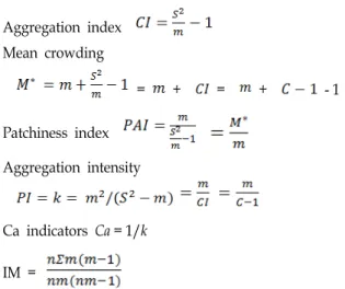
Table 2. Changes in gathering strength of Doellingeria scabra at different sampling quadrat sizes
Quadrat size (m×m) Aggregation or dispersion indices
C ID Z PI Distribution pattern
2×2 2×4 4×4 4×8 8×8 8×16 16×16 16×32 Mean
0.649 0.641 0.988 0.992 1.259 1.271 1.250 1.290 1.043
24.667 30.148 39.503 60.532 117.104 149.944 172.458 229.693 103.006
-1.636 -1.879 0.004 0.003 1.702 1.988 1.990 2.592 0.560
-1.073 -1.417 -51.949 -85.246 3.228 2.899 2.664 2.926 -15.996
Uniform Uniform Uniform Uniform Uniform Aggregation Aggregation Aggregation
-
Table 3. Clouding or patchiness indices of Doellingeria scabra at different sampling quadrat sizes
Quadrat size (m×m)
No.
Quadrat
Clouding or patchiness indices
M* PAI IM
2×2 2×4 4×4 4×8 8×8 8×16 16×16 16×32 Mean
32 16 12 8 6 4 4 2 10.5
0.026 0.150 0.633 1.007 0.647 1.096 1.056 0.916 0.691
0.068 0.294 0.981 0.007 0.988 1.310 1.345 1.376 0.796
0.073 0.307 1.019 1.021 0.999 1.327 1.359 0.480 0.823 the standard normal deviation (SND) for the plant genotype,
g (k) = {I (k) - u1}/u21/2, asymptotically has a standard nor- mal distribution [5]. Hence, SND g(k) values exceeding 1.96, 2.58, and 3.27 are significant at the probability levels of 0.05, 0.01, and 0.001, respectively.
Results
The optimum sample size is the smallest number of sam- ple units that would satisfy the objectives of the sampling program and achieve the desired precision of estimates. Each type of joined individuals and for each distance class of sep- aration were tested for significant deviation from random expectations by calculating the standard normal deviation.
No significant population structure of D. scabra was found within the 2.0 m quadrate sizes. Population densities (D) of D. scabra populations at Mt. Maebong varied from 0.35 to 2.97, with a mean of 2.94 (Table 1). Small quadrate sizes such as 2×2 m2, 2×4 m2, and 4×4 m2 have relatively high D values (>2), whereas larger or wider quadrate sizes such as 8×16 m2, 16×16 m2, and 16×32 m2 have, comparatively, very low D values (<1). The values (R) of spatial distance (the rate of observed distance-to-expected distance) among the near- est individuals were higher than 1 and the significant index of CR was >2.58. If by this parameter, the six scale plots (2×2 m2, 2×4 m2, 4×4 m2, 4×8 m2, 8×8 m2, and 8×16 m2) of D. scabra at Mt. Maebong were uniformly distributed in the forest community. However, D. scabra was aggregately dis- tributed in two large scale plots (16×32 m2 and 32×32 m2).
Eberhardt’s index of dispersion for point-to-organism dis- tances (IE) varied from 2.216 (2×4 m) to 3.704 (2×2 m2), with a mean of 2.623.
The values dispersion index (C) of D. scabra at Mt.
Maebong were lower at four scale plots (2×2 m2, 2×4 m2, 4×4 m2, and 4×8 m2) than 1 except four large scale plots
(8×8 m2, 8×16 m2, 16×16 m2, and 16×32 m2) (Table 2).
Departure from a random distribution can be tested by cal- culating the index of dispersion (ID). In this Model, values of ID ranged from 24.67 to 229.69. Large scale plots were considerably greater than those of small scale plots, indicat- ing that large scales plots tend to be aggregated. This ID index can be tested by Z value. If 1.96 ≥ Z ≥ -1.96, the spatial distribution would be random. Thus, the six scale plots (2×2 m2, 2×4 m2, 4×4 m2, 4×8 m2, 8×8 m2, and 8×16 m2) of D. scabra at Mt. Maebong were random distributed in the forest community. Two large plots (16x16 m2 and 16×32 m2) were aggregated (Z>1.96). Aggregation intensity (PI) ranged from -85.246 to 3.228 and it was not strong.
The mean crowding (M*) was 0.92(Table 3). The mean patchiness index (PAI) was 0.796. Both were showed positive values for all plots. The mean Morisita index (IM) was 0.82.
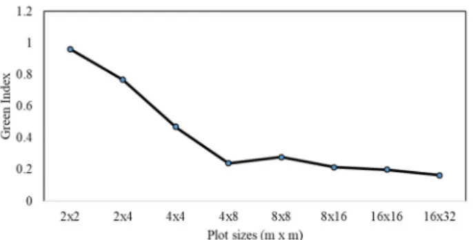
The values of δ were showed an overly steep slope at the plot 4×4 m2 (Fig. 1). The values of Morisita’s coefficient showed a tendency to decrease as the plot size increased (Fig. 2).
The spatial auto coefficient, Moran's I is presented in Table 4. Separate counts for each type of joined individuals
Fig. 1. The mean aggregation number to find the reason for the aggregation of Doellingeria scabra.
Fig. 2. The curves of patchiness in two areas of Doellingeria sca- bra using values of Green index.
Table 4. Spatial autocorrelation coefficients (Moran's I) among plots of Doellingeria scabra for eight distance classes
I II III IV V VI VII VIII
0.486*** 0.403*** 0.292* 0.274* 0.113 -0.053 -0.166* -0.234**
*: p<0.05, **: p<0.01, ***: p<0.001.
and for each distance class of separation were tested for sig- nificant deviation from random expectations by calculating the SND. Moran's I of D. scabra significantly differed from the expected value in 6 of 8 cases (75.0%). The first five classes were positive. Four of them showed significance, in- dicating similarity among individuals in the first four dis- tance classes (I~IV), i.e., pairs of individuals can separate by more than 8.0 m. Three of these values (37.5%) were neg- ative, indicating a partial dissimilarity among pairs of in- dividuals at the VI distance class scales (10-12 m).
Discussion
Thus, two large plots (16×16 m2 and 16×32 m2) of D. scabra at Mt. Maebong were clustered based on the Neatest Neighbor Rule (Table 1). The result of one plot (8×16 m2) in Table 2 was inconsistent with the previous results (Neatest Neighbor Rule). One of the reasons is in uneven
collection and distribution pattern of the D. scabra was quad- rat-sampling dependent. As Morisita’s coefficient estimates spatial distribution pattern using the mean and variance of each sampling date separately, so this index is more perfect than dispersion index [19]. The detailed knowledge of dis- persion in different time intervals during growing season would be useful for research strategies more than manage- ment programs.
The comparison of Moran’s I values to a logistic re- gression indicated that a highly significant percentage of in- dividual dispersion in D. scabra populations at Mt. Maebong could be explained by isolation by distance (Table 4).
The expected value of IE in a random population is 2.62 (Table 1). IE values for all quadrates are larger than 1.27.
Under the hypothesis, D. scabra is clumping. Clumped dis- persion is often due to an uneven distribution of nutrients or other resources in the environment. Species interactions can be intra- or interspecific. The former is usually negative due to conspecific competition for the same resources [14], while the latter can be negative (interspecific competition), positive (facilitation) or neutral.
Although positive interspecific interactions are not rare, the positive interaction often occurs because one species ameliorates a physical, physiological or trophic stress that otherwise compromises the fitness of a resource exploiter [16]. Also during extreme events which drive much of the gap formation in plant communities, species interactions take place and more importantly influence the survival of individuals [26]. In a high density plots, interspecies com- petition is maintained within a certain distance (Table 1).
However, in less dense plots, D. scabra could co-aggregate with each other to compete with other species.
M* was proposed by Lloyd to indicate the possible effect of mutual interference or competition among individuals [19]. As an index, mean crowding is highly dependent upon both the degree of clumping and population density. Patch- based measures of pattern include size, number, and density of patches [12]. Useful edge information may include perim- eter of individual patches, total perimeter of all patches of a particular class, the frequency of specific patch adjacencies, and various edge metric that incorporate the contrast (degree
of dissimilarity) between the patch and its neighbors.
However, different spatial patterns may also reflect differ- ential abilities of species to survive intra and interspecific competition during succession [9]. The effects of density-de- pendent mortality may be revealed by comparing the change in spatial pattern of different life-history stages [18, 21].
Conclusion, M* and PAI showed positive values for all plots. When the three indices C, M*, PAI were <1 and their values of PI were also shown smaller than zero, it means uniform distributed. In D. scabra, the two indices, C, PAI were >1 and their values of PI were also shown greater than zero, thus it means aggregately distributed. In many near neighbor plants of D. scabra at Mt. Maebong, density be- tween neighboring individuals was high and similarity was high. Whereas, two large plots (16×16 m2 and 16×32 m2) of D. scabra were clustered each other and aggregation. This plant is distributed in low mountains and is easy to collect.
The genetic resources can be secured by preserving the sizes of the effective group of this plant. According to the results of this study, the size of the D. scabra population should be at least 8×8 m2.
References
1. Arbous, A. G. and Kerrich, J. E. 1951. Accident statistics and the concept of accident proneness. Biometrics 7, 340-342.
2. Austin, M. P. 2002. Spatial prediction of species distribution:
an interface between ecological theory and statistical modelling. Ecol. Model. 157, 101-118.
3. Chung, T. Y., Eiserich, J. P. and Shibamoto, T. 1993. Volatile compounds isolated from edible Korean chamchwi (Aster scaber Thunb). J. Agric. Food Chem. 41, 1693-1697.
4. Clark, P. J. and Evans, F. C. 1954. Distance to nearest neigh- bor as a measure of spatial relationships in populations.
Ecology 35, 445-453.
5. Cliff, A. D. and Ord, J. K. 1971. Spatial Autocorrelation, pp.
178, Pion, London, England.
6. Dale, M. R. T. 1999. Spatial Pattern Analysis in Plant Ecology, pp. 326, Cambridge: Cambridge University Press, Cam- bridge, England.
7. Eberhardt, W. R. and Eberhardt, L. 1967. Estimating cotton- tail abundance from livertrapping data. J. Wild. Manage. 31, 87-96.
8. Fortin, M. J. and Dale, M. R. T. 2005. Spatial Analysis: A Guide for Ecologists, pp. 356, Cambridge University Press, Cambridge, England.
9. Getzin, S. and Wiegand, K. 2007. Asymmetric tree growth at the stand level: random crown patterns and the response to slope. Forest Ecol. Manag. 242, 165-174.
10. Greig-Smith, P. 1983. Quantitative Plant Ecology, pp. 359, 3rd ed. Blackwell Scientific, Oxford, USA.
11. Green, R. H. 1966. Measurement of non-randomness in spa-
tial distributions. Res. Pop. Ecol. 8, 1-7.
12. Gustafson, E. J. 1998. Quantifying landscape spatial pattern:
what is the state of the art? Ecosystems 1, 143-156.
13. Hines, W. G. S. and Hines, R. J. O. 1979. The Eberhardt index and the detection of non-randomness of spatial point distributions. Biometrika 66, 73-80.
14. Johnson, D. J., Beaulieu, W. T., Bever, J. D. and Clay, K.
2012. Conspecific negative density dependence and forest diversity. Science 336, 904-907.
15. Lian, X., Jiang, Z., Ping, X., Tang, S., Bi, J. and Li, C. 2012.
Spatial distribution pattern of the steppe toad-headed lizard (Phrynocephalus frontalis) and its influencing factors. Asian Herpet. Res. 3, 46-51.
16. Lio, J., Bogaert, J. and Nijs, I. 2015. Species interactions de- termine the spatial mortality patterns emerging in plant communities after extreme events. Sci. Rep. 5, doi:
10.1038/srep11229.
17. Lloyd, M. 1967. Mean crowding. J. Anim. Ecol. 36, 1-30.
18. Moeur, M. 1997. Spatial models of competition and gap dy- namics in old-growth Tsuga heterophylla / Thuja plicata for- ests. Forest Ecol. Manag. 94, 175-186.
19. Moradi-Vajargah, M., Golizadeh, A., Rafiee-Dastjerdi, H., Zalucki, M. P., Hassanpour, M. and Naseri, B. 2011. Popula- tion density and spatial distribution pattern of Hypera postica (Coleoptera: Curculionidae) in Ardabil, Iran. Not. Bot. Horti.
Agrobo. 39, 42-48
20. Patil, G. P. and Stiteler, W. M. 1974. Concepts of aggregation and their quantification: a critical review with some new results and applications. Res. Popul. Ecol. 15, 238-254.
21. Plotkin, J. B., Chave, J. and Ashton, P. S. 2002. Cluster analy- sis of spatial patterns in Malaysian tree species. Am. Nat.
160, 629-644.
22. Pommerening, A. and Särkkä, A. 2013. What mark vario- grams tell about spatial plant interactions. Ecol. Model. 251, 64-72.
23. Shaukat, S. S., Aziz, S., Ahmed, W. and Shahzad, A. 2012.
Population structure, spatial pattern and reproductive ca- pacity of two semi-desert undershrubs Senna holosericea and Fagonia indica in southern Sindh, Pakistan. Pak. J. Bot. 44, 1-9.
24. Sokal, R. R. and Oden, N. L. 1978a. Spatial autocorrelation in biology 1. Methodol. Biol. J. Lin. Soc. 10, 199-228.
25. Sokal, R. R. and Oden, N. L. 1978b. Spatial autocorrelation in biology 2. Some biological implications and four applica- tions of evolutionary and ecological interest. Biol. J. Lin. Soc.
10, 229-249.
26. Stachowicz, J. J. 2001. Mutualism, facilitation, and the struc- ture of ecological communities. Bioscience 51, 235-246.
27. Thiruvengadam, M., Praveen, N., Yu, B., Kim, S. and Chung, I. 2014. Polyphenol composition and antioxidant capacity from different extracts of Aster scaber. Acta Biol. Hung. 65, 144-155.
28. Zhang, Y. T., Li, J. M., Chang, S. L., Li, X. and Lu, J. J.
2012. Spatial distribution pattern of Picea schrenkiana pop- ulation in the Middle Tianshan Mountains and the relation- ship with topographic attributes. J. Arid Land 4, 457-468.
초록:한국 매봉산 참취의 공간적 분포 양상과 집단 구조 이병룡1․허만규2*
(1서원대학교 생물교육과, 2동의대학교 식품공학과)
참취, Doellingeria scabra Thunb. (이전의 학명: Aster scaber Thunb.)는 국화과의 다년생 초본으로 한국의 야생 산지에서 흔히 찾을 수 있다. 본 연구는 강원도 태백시 매봉산에 분포하는 참취의 국지적 집단에 대해 패치 특성 을 측정하고자 하였다. 이 종의 공간적 분포를 평가하기 위해 분산의 지수, Lloyd 평균 군집도, Morisita 지수 등을 통해 자료를 분석했다. 참취 집단의 평균 밀도는 2.94이었다. 참취는 작은 규모의 플롯에서는 일정한 분포 또는
임의 분포를 하였고, 두 개의 큰 규모 플롯(16×32 m2와 32×32 m2)에서는 응집 형태로 분포했다. 평균 밀집도(M*)
는 0.916이었다. 평균 patchiness index (PAI)는 0.796이었다. Morisita의 계수는 플롯 크기가 커짐에 따라 감소하는 경향을 보였다. 이 집단에서 Eberhardt 지수(IE)의 예상 값은 2.623이었다. 참취의 Moran's I 값에서 처음 5개 구간 은 양의 값이었다. 그 중 4개는 유의성을 나타내어 개체간 유사성은 8 m 이내에서 발생한다고 볼 수 있다. 본 연구는 매봉의 참취군락뿐만 아니라 다른 산의 산림 생태계 내 참취 군락의 지속 가능한 유지 및 복원에 대한 이론적 근거를 제공할 수 있다.