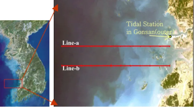
Fig. 1. Study area: color composite image (Red-3; Green-2; Blue-1) of Landsat5 TM (21-05-1999) with two profile lines. : line-a (the profile-line from Mankyeng river area) and line-b (the profile-line from Dongjin river area)
Monitoring suspended sediment distribution using Landsat TM/ETM+ data
in coastal waters of Seamangeum, Korea
Jee-Eun Min1,2*, Joo-Hyung Ryu1, Shanmugam P.1, Yu-Hwan Ahn1, and Kyu-Sung Lee2
1Satellite Ocean Research Lab., Korea Ocean Research & Development Institute Ansan P.O. Box 29, SEOUL 425-600, South Korea
2Department of Geoinformatic Engineering, INHA University Abstract: Since the tide embankment construction started in
1991, the coastal environment in and around the Saemangeum area has undergone changes rapidly, there is a need for monitoring the environmental change in this region. Owing to high temporal and spatial heterogeneity of the coastal ecosystem and processes as well as the expense with traditional filed sampling at discrete locations, satellite remote sensing measurements offer a unique perspective on mapping a large region simultaneously because of the synoptic and repeat coverage and that quantitative algorithms used for estimating constituents’ concentration in the coastal environments. Thus, the main objectives of the present study are to analyze the retrieved Suspended Sediment (SS) pattern to predict changes after the commencement of the tide embankment construction work in 1991. This is accomplished with a series of the Landsat TM/ETM+ imagery acquired from 1985-2002 (a total of 18 imageries). Instead of a simple empirical algorithm, we implement an analytical SS algorithm, developed by Ahn et al. (2003), which is especially developed for estimating SS concentration (SSC) in Case-2 waters. The results show that there is a significant change in SS pattern, which is mainly influenced by the tide and tidal height after the construction of the embankment work. As the construction progressed, the distribution pattern of SS has greatly changed, and the rate of SS concentration in the gap area of the dyke of post-construction has significantly increased.
Keywords: Suspended Sediments (SS), SS algorithm, Landsat TM/ETM+, Seamangeum
1. Introduction
Determination of suspended sediment (SS) in coastal waters is essential because it is one of the major environmental parameters of water and is a good tracer of water movement and transport of suspended materials and pollutants. In coastal construction such as tide embankment, understanding of the movement and transportation of coastal suspended sediment (SS) is very important in many problems related to water quality, tidal erosion, modification of harbor basins and change of coastal environment. In Seamangeum area, a large-scale reclamation project is being carried out for the effective use of land for agriculture purposes. As a
result, there was a significant change in coastal environments of this region, so several studies of water quality, ecology, geology and hydrography for monitoring of the sea area environmental change. In this study, we assess changes in SS distribution of the pre- and post construction of the Seamangeum embankment using satellite remote sensing technique.
2. Study area
The Samangeum is situated in the western coast tract of Korea, where Mankyung and Dongjin rivers discharge fresh water. In this area, Saemangeum tidal dyke of 33 km long is now in the course of construction for reclaiming the very shallow estuary region of 41,000ha. Thus, it is necessary to monitoring a series of environmental changes induced by man-made activities.
At present, the dyke connected with Gogunsan-Gundo separates this area into three regions; northwestern, southwestern and eastern (Saemangeum) region of the dyke and the water in Saemangeum region is exchanged through one gap in the northern dyke and two gaps in the southern dyke. To monitor SS distribution in three parts of the dyke, we analyze two profile lines on the northern and southern gap (Fig. 1).
Line-a
Line-b
Tidal Station in Gonsan(outer)
3. Methodology
1) Data set
In this study, a series of Landsat TM/ETM+ imagery acquired from 1985 – 2002 (a total of 18 imageries) were used for monitoring SS distribution in the Seamangeum coastal waters (Table 1). Of these, 14 images were acquired at the ebb tides and the rest at flood tides. For the geometric correction of the image, we adopted image-to-image registration method: firstly, IRS image was geometrically corrected with respect to digital map, and then TM image was geo-corrected according to the IRS image. The images were co- registered by taking about 15 GCPs from the urban area and surrounding islands. The registration accuracy achieved was less than 0.5 pixel RMS using the nearest neighborhood resampling method. The main intention of adopting this method is that it does not alter the pixel values (Jensen, 1996).
Table 1. List of the Landsat TM/ETM+ imagery used in this study.
Data satellite date local time Tide Tide height(cm) No. sensor (yyyy/mm/dd) Condition* (location)*
1 Landsat TM 1985/10/21 10:40:20 ebb-middle 368 2 Landsat TM 1990/07/31 10:31:28 ebb-start 469 3 Landsat TM 1992/06/02 10:34:58 ebb-end 117 4 Landsat TM 1992/09/22 10:33:24 flood-end 505 5 Landsat TM 1993/10/27 10:33:34 flood-middle 344 6 Landsat TM 1996/05/12 10:22:21 flood-end 563 7 Landsat TM 1998/11/26 10:50:28 ebb-middle 295 8 Landsat TM 1998/12/28 10:50:31 ebb-start 537 9 Landsat TM 1999/05/21 10:49:47 ebb-middle 413 10 Landsat TM 1999/11/13 10:47:14 ebb-end 157 11 Landsat TM 2000/05/07 10:47:03 ebb-end 143 12 Landsat TM 2000/10/30 10:50:13 ebb-end 58 13 Landsat ETM+ 2000/11/23 11:01:31 flood-middle 413 14 Landsat ETM+ 2001/03/31 11:01:36 ebb-middle 309 15 Landsat ETM+ 2001/04/16 11:01:20 ebb-middle 464 16 Landsat ETM+ 2001/09/23 10:59:41 ebb-middle 244 17 Landsat ETM+ 2001/11/10 10:59:40 ebb-start 497 18 Landsat ETM+ 2002/02/14 11:00:21 ebb-end 44
*Referred to tide register at Gunsan Tidal Station (outer) (fig. 1) from NORI (National Oceanographic Research Institute)
2) Radiance and reflectance conversion
To convert digital numbers (DN) of the original image to radiance at the satellite level (Lsat), the following equation was used:
rescale cal
rescale
sat G Q B
L = × + (1) Where, G and B are gain and bias of a given spectral band, respectively. Then radiance was converted to reflectance (R) according to the following equation given by Chavez (1996):
τ π
θ π
∗
∗
−
∗
∗
= −
)) 180 / ) 90 ((
(
)
( 2
COS E
D L R L
o
atm
sat (2)
where, Latm = Atmospheric path radiance; D = Normalized Earth-Sun Distance; E = Solar spectral o irradiance on a surface perpendicular to the sun ray’s outside the atmosphere; θ = Solar zenith angle; τ = Atmospheric transmittance.
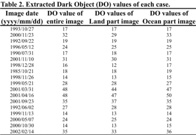
Table 2. Extracted Dark Object (DO) values of each case.
Image date (yyyy/mm/dd)
DO value of entire image
DO values of Land part image
DO values of Ocean part image
1993/10/27 17 17 17
2000/11/23 32 29 33
1992/09/22 19 19 19
1996/05/12 24 25 25
1990/07/31 17 18 17
2001/11/10 31 30 31
1998/12/28 16 12 17
1985/10/21 18 18 19
1998/11/26 14 13 15
1999/05/21 28 28 27
2001/03/31 48 44 47
2001/04/16 48 47 50
2001/09/23 35 37 35
1992/06/02 27 28 28
1999/11/13 14 13 14
2000/05/07 24 25 24
2000/10/30 14 13 15
2002/02/14 35 33 36
Path radiance was corrected by using Dark Object Subtraction (DOS) technique as given by Chavez (1988), who used the histogram method for extracting a dark object from the Landsat 5 TM image. It is superior to use the entire image for the extraction of the Dark Object (DO) for land applications. However, this method of deriving a dark object is no longer invalid in the case of ocean applications, because DO value of entire image is lower than using ocean part (Table 2), so it often leads to an underestimation of the atmospheric path signal. Thus, we used image pixels of the ocean part for extracting the DO. Correction for atmospheric transmission was performed according to the Cosine of Solar Zenith Angle (COST) model given by Chavez (1996).
3) Implementation of SS Algorithm
To estimate SSC in the Samangeum coastal waters, we used SS algorithm that has been developed based on the remote sensing reflectance (Rrs) model, developed by Ahn (1999). Rrs model is based on the functions of inherent optical properties such as absorption [a(λ)] and backscattering [bb(λ)] coefficients of six water components including water, phytoplankton (chl), dissolved organic matter (DOM), suspended mineral particles (SS), heterotropic organism (he) and an unknown component, possibly represented by bubbles or other particulates unrelated to the first five components. Based on these variables, the author obtained the following relationship
) 044(
.
0
∑ ∑ ∑
= +
bi i
bi
rs a b
R b (3)
(a) (b)
(c) (d)
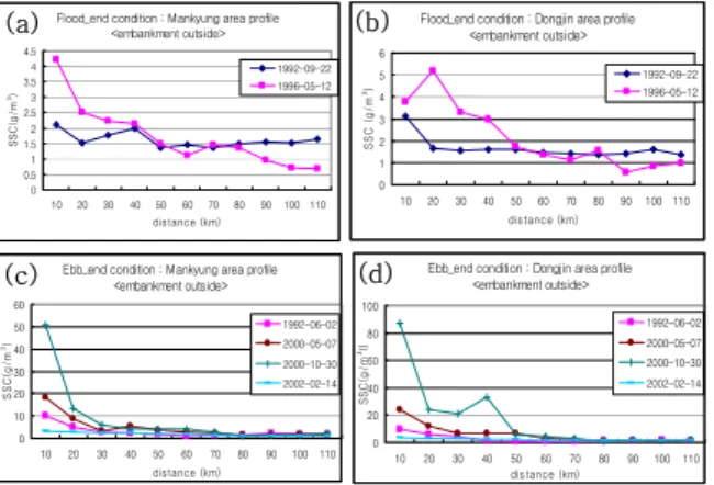
Fig. 3. SS distribution map at flood and ebb end condition according to construction.
(a) Before construction at flood end condition in 1992/09/22 (b) After construction at flood end condition in 1996/05/12 (c) Before construction at ebb end condition in 1992/06/02 (d) After construction at ebb end condition in 2000/05/07 Compare with in-s itu data
<over 70 km dis tance >
0 0.5 1 1.5 2 2.5 3 3.5 4 4.5 5
70 80 90 100 110
distance (km) SSC(g/m3)
1992-06-02 2000-05-07 2000-10-30 2002-02-14 1985-10-21 1999-05-21 2001-03-31 2001-04-16 2001-09-23 1990-07-31 2001-11-10 1992-09-22 1996-05-12 1993-10-27 2000-11-23 2001-06 in s itu data
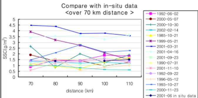
Fig. 2. Compare off-shore sea site SSC with in situ data
The modeled Rrs values were converted to the equivalent remote sensing reflectance at the TM bands and related to SSC to derive SS algorithm. The general form of SS algorithm is given as
B A
B m g
SS> = −
< [ / 3] [ 2(λ)] (4) where, B2(λ) : the weighted Rrs values for TM band2, A and B : regression coefficients. The conversion is accomplished by the following expression,
) ( ...
) ( ) (
) ( ) ( ...
) ( ) ( ) ( ) ) ( (
2 1
2 2 1 1 2
n
n rs n rs
rs
S S
S
R S R
S R B S
λ λ
λ λ λ λ λ
λ λ λ
+ + +
× + +
× +
= × (5)
where, S(λ) : the TM spectral responsivity, Rrs(λ) : the remote sensing reflectance at 2nm intervals for a given waveband, n : the number of spectral responsivity or Rrs
for a given TM waveband. A statistical regression analysis of the remote reflectance data was performed against the SSC to derive SS algorithm. According to Ahn et al. (2003), the empirical formula derived to estimate SSC is given as follows
e x
m g
SS>( / 3)=0.99 199.9
< (6)
where, x refers to Rrs(TM band 2). The exponential form is due to the fact that the total suspended sediment concentration corresponds best with an exponential, rather than linear function of radiance or reflectance (Klemas et al. 1974).
4. Results
1) Confirmation SSC result using in situ data
In order to evaluate the performance of SS algorithm, we compared the retrieved SSC with in-situ SSC of the same area. Although we don’t have any field measurements to coincide with satellite images, we compared the general SS distribution in the outer shelf areas (70 km away from the shore), where the variations in SSC is minimum. Even if the time of field measurement doesn’t coincide with that of images, the result indicates that the retrieved SSC is comparatively well consistent with the in-situ data. In contrast, there occurs a significant discrepancy between the retrieved
and measured values in areas close to the coast (less than 30km). In a few images, the SSC values are particularly very high. The reasons are attributed to several factors: firstly, atmospheric correction is unsuccessful with the DO, because having adopted this DO value underestimates the atmospheric path signal.
Moreover, extraction of DO in ocean is very difficult.
Unlike the land, there is no shadow in the ocean, so clear water pixel value has still few reflectance that is generally assumed as DO value. One should note that the west sea of Korea is typically of Case-2 water, so there is no pixel value considered to be DO for removing the atmospheric effects. Besides the ocean reflectance, other effects such as Fresnel and white cap reflectance are also significant and must be removed effectively.
The other reason for the overestimation of SSC in coastal areas is bottom reflection effect. The areas with water depth less than 30m have multi-reflectance that is the sum of water and bottom. In this case, the high reflectance leads to an essential overestimation of the calculated SSC. Because of the above reasons, the DOS method is unsuitable and process to mask out the sites of less than 30m water depth are needed.
2) SS distribution changes according to dyke construction.
According to the construction of dyke, SS distribution pattern has much changed. Generally, SSC of the post-construction work appears to be significantly higher than that of the pre-construction.
During the flood tides, SS distribution of the pre- construction is nearly similar in all areas of upper and lower Gogunsan-Gundo with triangular shape, while it is much higher inside of dyke of the post-construction (Fig. 2a and b). And during the end tide conditions, the SS distribution of pre-construction is similar to that of
Flood_end condition : Mankyung area profile
<embankment outside>
0 0.5 1 1.5 2 2.5 3 3.5 4 4.5
10 20 30 40 50 60 70 80 90 100 110 dis tance (km) SSC(g/m3)
1992-09-22 1996-05-12
Flood_end condition : Dongjin area profile
<embankment outside>
0 1 2 3 4 5 6
10 20 30 40 50 60 70 80 90 100 110
distance (km) SSC (g/m3)
1992-09-22 1996-05-12
Ebb_end condition : Mankyung area profile
<embankment outside>
0 10 20 30 40 50 60
10 20 30 40 50 60 70 80 90 100110
distance (km) SSC(g/m3)
1992-06-02 2000-05-07 2000-10-30 2002-02-14
Ebb_end condition : Dongjin area profile
<embankment outside>
0 20 40 60 80 100
10 20 30 40 50 60 70 80 90 100 110
dis tance (km) SSC(g/m3l)
1992-06-02 2000-05-07 2000-10-30 2002-02-14
Fig. 4. Profile analysis in line-a (Mankyung River) and line-b (Dongjin River)
the flood tide conditions, but it is much higher in the gap area of the dyke of the post-construction. The effects of down-welling current induce changes in the direction of SS distribution from the northeast to southwest (Fig. 2c and d). These were confirmed with profile analysis. Two profiles made between Mankyung (line-a) and Dongjin River (line-b) (Fig. 1) indicate high SSC of the post-construction. Exceptionally, at ebb condition (14-02-2002) the SSC values are low on the whole. The reason is because of an underestimation of the atmospheric path signal.
5. Conclusions
In this study, we carried out an extensive analysis for assessing and monitoring the rate of change in SS distribution according to dyke construction in the Seamangeum area using Landsat images. From this analysis, it is inferred that SSC of post-construction is much higher than that of the pre-construction. As the dyke construction continued to progress, the SSC in the gap area has significantly increased.
The SS algorithm and atmospheric correction presented in this paper is sufficient for assessing and monitoring the changes in SS distribution patterns in and around the study site. However, they must be improved and validated before extending for other qualitative applications. The estimated SSC using SS algorithm needs to be confirmed with in-situ measurements. In the case of atmospheric correction, an efficient method needs to be developed, because the DOS method produces significant errors in terms of underestimating the atmospheric path signal over the ocean. To solve these problems, we are now developing new and more efficient methods for analyzing remotely sensed data in ocean applications.
6. References
[1] Ahn, Y. H., 1999. Development of an inverse model from ocean reflectance, Marin Technology Society
Journal, 33 : pp. 69-80.
[2] Ahn, Y. H., J. E. Moon, and S. Gallegos, 2001.
Development of suspended particulate matter algorithms for ocean color remote sensing, Korean Journal of Remote Sensing, 17 : 285-295.
[3] Ahn, Y. H., P. Shanmugam, and J. E. Moon, 2003.
Retrieval of ocean color from Multi-spectral Camera on Kompsat-2 for monitoring highly dynamic ocean features, Submitted for the International Journal of Remote Sensing.
[4] Chavez, P., 1988. An Improved Dark-Object Subtraction Technique for Atmospheric Scattering Correction of Multispectral Data, Remote Sensing of environment, 24 : pp. 459-479.
[5] Chavez, P., 1996. Image-based atmospheric corrections- Revisited and improved, Photogrammetry Engineering and Remote Sensing, 62 : pp. 1025-1036.
[6] Islam, M.R., S. F. Begum, Y. Yamaguchi, K. Ogawa, 2002. Distribution of suspended sediment in the coastal sea off the Ganges-Brahmaputra River mouth : observation from TM data, J. of marine systems, 32 : pp.
307-321.
[7] Lee, S.H., H.Y. Choi, Y.T. Son, H.K. Kwon, Y.K. Kim, J.S. Yang, H.J. Jeong and J.G. Kim, 2003. Low-salinity water and circulation in summer around Saemangeum Area in the West coast of Korea, Journal of the Korean Society of Oceanography, 8(2) : pp. 138-150.
[8] Lee, H.J., E.S. Kim, H.G. Kim, G.J. Lee, G.I. Jang, C.H.
Cho, Integrated preservation study on the oceanic environments in the Saemangeum Area(1st year), Ministry of Maritime Affairs & Fisheries
[9] Lee, H.J. et al., A pilot study on Suspended Sediments transport around the Saemankeum dyke in terms of construction of artificial tidal flat, Korea Ocean Research Division Institute (KORDI).
[10] Li, R. R., Y. J. Kaufman, B. C. Gao, C. O. Davis, 2003.
Remote Sensing of Suspended Sediments and Shallow Coastal Waters, IEEE transactions on geoscience and remote sensing, 41(3) : pp. 559-566.
[11] Jensen J.R., 1996. Introductory digital image processing : A remote sensing perspective (2nd edition), Prentice Hall, New jersey.
(a) (b)
(c) (d)