RECEIVING TIME CALCULATION METHODS FOR LINES OF COMS MI LV1B IMAGES
Seok-Bae SEO and Sang-Il AHN
Korea Aerospace Research Institute
115 Gwahangno, Yuseong-Gu, Daejeon, Republic of Korea E-mail : [email protected], [email protected]
ABSTRACT: MI LV1B images has no time information per each line, but weather prediction using the MI LV1B images needs time information on that. This paper proposes two feasible methods of receiving time calculation on lines of MI LV1B images, and describes analyses results for two methods using a simulated data.
KEY WORDS: COMS, Level 1B Image, Receiving Time, Re-sampling Grid, and Simulated Data.
1.
INTRODUCTION
COMS (Communication Ocean and Meteorological Satellite) has two imagers, MI (Meteorological Imager) and GOCI (Geostationary Ocean Colour Imager) for Earth observation. For the MI, transmitted data to ground station are used for a weather forecasting after its processing in IMPS (Image Pre-processing Subsystem).
The IMPS generates 4 Level Products - Raw Data, LV0 Product, LV1A Product, LV1B Product - using received data from the COMS.
Scan line time information of LV1A IMG (COMS MI LV1A Image) can be simply decided using its receiving time-tag information, but that of LV1B IMG (COMS MI LV1B Image) is ambiguous because geometric correction processing inevitable for LV1B IMG includes inherently re-sampling functions.
This paper explains two possible receiving time calculation methods for lines of LV1B IMG from engineering’s point of view and describes difference analyses results for two methods using a simulated data.
For the first, formats of LV1A IMG and LV1B RSG are explained in chapter 2, and then two calculation methods of receiving time for lines of LV1B IMGs are described in chapter 3. Chapter 4 shows results using simulated data and chapter 5, the last part, is conclusions for this paper.
2.
FORMAT OF INPUT DATA
Input files, LV1A IMG and LV1B RSG, of the RTL1B (Receiving Time for Lines of COMS LV1B Images) are explained in this chapter.
2.1
LV1A IMG
Each line of LV1A IMG has line header which were included time of start and end as a count stamps, LLCS (Left Line Count Stamp) and RLCS (Right Line Count Stamp). Because that the MI gathers sequence of image lines for Earth images based on alternative moving of scan mirror, receiving time can be calculated using LLCS, RLCS, and scan direction (EW or WE) for each line of LV1A IMG.
LV1A IMG made up with successive sequences of LLCS, line image, and RLCS. Where, position of LLCS and RLCS can be exchanged each other by the scan direction.
2.2
LV1B RSG
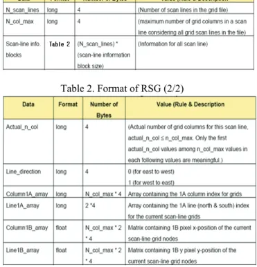
LV1 RSG contains relationship of re-sampling between LV1A IMG and LV1B IMG. Detailed format of LV1B RSG is described in Table 1 and 2. Contents in Table 1 are fixed sized, but ones of Table 2 are decided by size of LV1A/LV1B images and interval of re-sampling grids.
Table 1. Format of RSG (1/2)
Table 2. Format of RSG (2/2)
3.
CALCULATION AND ANALYSIS METHOD
Calculation and analysis methods of RTL1B are made
up following three steps, 3.1~3.3.
3.1
Receiving time calculation for lines of LV1A IMG The MI acquires images using alternative scan of EW or WE direction. For VIS (Visible) channel case, eight image lines are unit of one scan line acquisition. IMPS (Image Pre-processing Subsystem), a part of data processing system on ground, attaches LLCS and RLCS at front and end of each scan line. Figure 1 explains scan direction of the MI and meaning of LLCS/RLCS.
Data unit of the MI is 60 bytes DB (Data Block) which contains Earth images and MI telemetries. 5,460 DB are transmitted to ground (IMPS) per one second from the MI with 6.208 Mbps speed.
Figure 1. Earth scans and count stamps of the MI Time of start and end for an observation and its duration are calculated as following equation 1 to 4.
Receiving Duration of scan lines of LV1A IMG [sec]
= |LLCS-RLCS|/5,460 (1) STO (Time of start for observation) [HH:MM:SS]
= UTC
FP+ MIN({LLCS,RLCS})/5,460 (2) ETO (Time of end for observation) [HH:MM:SS]
= UTC
FP+ MAX({LLCS,RLCS})/5,460 (3) DO (Duration for observation) [sec]
= ETO – STO (4)
Where, MIN/MAX means decision function for maximum/ minimum values, UTC
FPimplies UTC of the first pixel receiving for each observation (HH:MM:SS), and ‘{}’ is a set of data.
3.2
RTL1B calculation using LV1B RSG
RTLIB calculation using LV1B RSG should be considered that each line of LV1B IMG related with several LV1A image lines which are included in a line of LV1B IMG. Thus one line selection of LV1A IMG for a line of LV1B IMG is needed.
This paper uses the fastest line of LV1A IMG as a related one with a line of LV1B IMG. In addition, line numbers of LV1B IMG are floating point values in LV1B RSG, so floating point values are rounded to integer ones.
3.3
RTL1B calculation using STO and ETO
Even though eight image lines are unit of LV1A IMG by scans of the MI, unit of RTL1B calculation using STO and ETO is based on one image line. After that a linear interpolation is used at the RTL1B calculation using STO and ETO.
Because that part of lines of LV1A IMG, not entire one, are involved re-sampling processing using LV1A IMG and LV1B IMG, DO (observation duration of LV1A IMG) is larger than receiving time of LV1B IMG’s observation duration.
4.
ANALYSES RESULTS
The MI has five observation modes; FD: Full Disk, LA: Local Area, ENH: Extended North Hemisphere, APNH : Asian Pacific North Hemisphere, and LSH : Limited South Hemisphere.
Five observation data were selected for this test from MI WBL3 data, simulated data for COMS, as following Table 3.
Table 3. Test Data
Mode Image Reference Image Lines (Scan Lines) FD 2011-03-21.23-45-20 11,160 (1,395) LA 2011-03-22.00-13-12 1,192 (149) ENH 2011-03-22.00-15-20 6,352 (794) APNH 2011-03-22.00-30-20 3,240 (405)
LSH 2011-03-22.00-35-20 3,360 (420) Because information of VIS image and IR (Infra Red) are included together in same DB (active scan block), only VIS channel data are analyzed for the test, hereafter.
4.1
Receiving time for lines of LV1A IMG
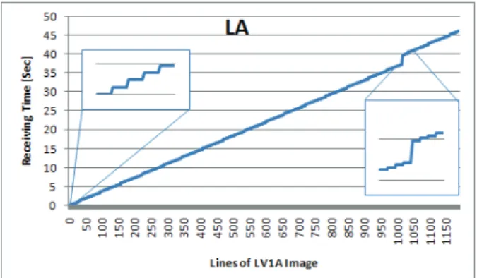
Figure 2 shows receiving time for lines of LV1A IMG
using LLCS and RLCS.
Figure 2. Receiving time for lines of LV1A IMG The smaller stair type increases (between 10 and 20 lines in LA mode) were founded at entire LV1A IMG which were related with unit of VIS channel (8 lines) for the MI scan operation. The larger variations in LA, ENH, APNH, and LSH were effects from space look among Earth imaging in the MI scan operation.
Table 4 describes results of receiving time information for each observation; STO, ETO, and DO. For the convenience of RTL1B calculation, STOs were set to 00:00:00 for each observation.
Table 4. STO, ETO, and DO of LV1A IMGs
Mode STO ETO DO [sec]
FD 00:00:00 00:27:06 1626.078022 LA 00:00:00 00:00:46 46.032601 ENH 00:00:00 00:12:08 728.455678 APNH 00:00:00 00:03:55 235.451282
LSH 00:00:00 00:06:23 382.986081
4.2
RTL1B calculation using LV1B RSG
Figure 3 shows one of result of RTL1B calculation using LV1B RSG (LA mode). The result was similar with Figure 2 one, but there is no stair type increases. Because that the result includes re-sampled lines, not entire lines of LV1B IMG.
4.3
RTL1B calculation using STO and ETO
Figure 4 shows one of result of RTL1B calculation using STO and ETO (LA mode). Because that linear interpolation are used this calculation, there is no stair type increases.
4.4
Results comparison of two RTL1B calculations:
‘using LV1B RSG’ vs. ‘using STO and ETO’
Differences between two RTL1B calculations (using LV1B RSG vs. using STO and ETO) were described in this chapter. Figure 5 shows comparison results for two RTL1B calculations and those differences, and Table 5 describes those maximum differences.
Figure 3. RTL1B calculation using LV1B RSG
Figure 4. RTL1B calculation using STO and ETO
Figure 5. Comparisons of two RTL1B calculations.
Table 5. Max. Differences for two RTL1B calculations Mode DO [Sec] Max. Diff [Sec]
FD 1626.078022 11.94
LA 46.032601 4.20
ENH 728.455678 9.05
APNH 235.451282 6.84
LSH 382.986081 9.77
Because that part of lines of LV1A IMG, not entire one, are involved re-sampling processing, receiving time duration of OT(STO and ETO) methods were larger than that of LV1B RSG methods.
The maximum difference of this calculation is 11.94 sec for the FD mode analysis.
5.
![Table 5. Max. Differences for two RTL1B calculations Mode DO [Sec] Max. Diff [Sec]](https://thumb-ap.123doks.com/thumbv2/123dokinfo/5192519.602448/4.892.89.430.121.290/table-max-differences-rtl-calculations-mode-sec-diff.webp)
