Estimation for the Double Exponential Distribution Based on Type-II Censored Samples
Suk-Bok Kang1)․Young-Suk Cho2)․Jun-Tae Han3)
Abstract
In this paper, we derive the approximate maximum likelihood estimators of the scale parameter and location parameter of the double exponential distribution based on Type-II censored samples. We compare the proposed estimators in the sense of the mean squared error for various censored samples.
Keywords : Approximate maximum likelihood estimator, Double exponential distribution, Type-II censored sample
1. Introduction
Consider the double exponential or Laplace distribution with the probability density function (pdf)
f( x ;θ,σ) = 1
2σ e- |x - θ |/σ
, - ∞ < x < ∞ , σ > 0 , (1.1) and the cumulative distribution function (cdf)
F( x ;θ,σ) =
{ 1 -1212expexp[-[-θ - xσx - θσ ],], x≥θ. x≤θ, (1.2)
1) First Author : Professor, Department of Statistics, Yeungnam University, Gyongsan, 712-749, Korea
E-mail : [email protected]
2) Assistant professor, School of Free Major, Miryang National University, Miryang, 627-702, Korea
3) Graduate student, Department of Statistics, Yeungnam University, Gyongsan, 712-749, Korea
The double exponential distribution is used to model symmetric data with long tails. This distribution also arises directly when a random variable occurs as the difference of two variables with exponential distributions with the same scale.
Govindarajulu (1966) gave the coefficients of the best linear unbiased estimators for the location and the scale parameters in the double exponential distribution from complete and symmetric censored samples. Raghunandanan and Srinivasan (1971) presented some simplified estimators of the location and the scale parameters of a double exponential distribution. Bain and Engelhardt (1973) discussed the usefulness of the double exponential distribution as a model for statistical studies, and obtained the confidence intervals based on the maximum likelihood estimators for the location and the scale parameters of a double exponential distribution, and Kappenman (1975) obtained the conditional confidence intervals for the parameters of a double exponential distribution. Shyu and Owen (1986a, 1986b) obtained the tolerance intervals for the two-parameter double exponential distribution.
The approximate maximum likelihood estimation method was first developed by Balakrishnan (1989) for the purpose of providing the explicit estimators of the scale parameter in the Rayleigh distribution. Kang (1996) obtained the approximate maximum likelihood estimator (AMLE) for the scale parameter of the double exponential distribution based on Type-II censored samples and he showed that the proposed estimator is generally more efficient than the best linear unbiased estimator and the optimum unbiased absolute estimator. Kang et al. (1997) proposed the AMLE of the location and the scale parameters of the two-parameter exponential distribution with Type-II censoring. Childs and Balakrishnan (1996, 2000) developed the conditional inference procedures for the Laplace distribution based on conventionally Type-II right censored samples and the progressive Type-II censored samples.
In this paper, we derive the AMLEs of the scale parameter σ and the location parameter θ based on Type-II censored sample. We also compare the proposed estimators in the sense of the mean squared error (MSE) for various censored samples.
2. Approximate Maximum Likelihood Estimators
Let us assume that the following Type-II censored sample from a sample of size n is
Xr + 1:n≤ Xr + 2:n≤ … ≤ Xn - s :n (2.1)
where the first r and the last s observations are censored.
The likelihood function based on the Type-II censored sample in (2.1) is given by
L = n!
r!s! { F( Xr + 1:n)}r{ 1 - F( Xn - s :n)}s n - s∏
i = r + 1f( Xi :n). (2.2)
By putting Z i :n= ( Xi :n-θ )/ σ, the likelihood function can be rewritten as
L = n!
r!s! σ- A{ F( Zr + 1:n)}r{ 1 - F( Z n - s :n)}s ∏
n - s
i = r + 1f( Zi :n) (2.3)
where A = n - r - s is the size of the censored sample in (2.1), f( z) and F( z) are the pdf and the cdf of the standard double exponential distribution, respectively.
We have the log-likelihood function as follows;
ln L = ln( r!s!n! )- A ln σ + r ln { F( Zr + 1:n)} + s ln { 1 -F( Zn - s :n)} + ∑
n - s
i = r + 1lnf( Zi :n).(2.4) By realizing that f '( z)
f( z) = - |z |
z , z ≠ 0, on differentiating with respect to σ in turn and equation to zero, we obtain the estimating equation as
∂ ln L
∂ σ =- 1
σ[A +r F( Zf( Zr + 1:nr + 1:n)) Zr + 1:n- s 1 - F( Zf( Zn - s :nn - s :n) ) Zn - s :n-i = r + 1n - s∑ |Zi :n|]
= 0.
(2.5)
Equation (2.5) does not admit an explicit solution for σ. But we can expand the functions
f( Zr + 1:n)
F( Zr + 1:n) and f( Zn - s :n) 1 - F( Zn - s :n)
in Taylor series around the points
F- 1( pr + 1) ={ - ln { 2( 1 - pr + 1)}, pr + 1≥ 0.5 ln (2pr + 1), pr + 1< 0.5
(2.6)
and
F- 1( pn - s) ={ - ln { 2( 1 - pn - s)}, pn - s≥ 0.5 ln (2pn - s), pn - s< 0.5
(2.7)
where pi= i
n + 1 and qi= 1 - pi, respectively.
We also can expand the functions f(Z r + 1:n)
F( Zr + 1:n) Zr + 1:n and f(Z n - s :n)
1 - F( Zn - s :n) Zn - s :n
in Taylor series around the points (2.6) and (2.7), respectively. So we consider three cases as zr + 1:n≥ 0, zr + 1:n< 0 <zn - s :n, and zn - s :n≤ 0.
Balakrishnan and Cutler (1994) derived explicitly the maximum likelihood estimator of the parameter θ based on symmetrically Type-II censored samples as follows;
If Xr + 1 :n≤ θ ≤ Xn - r :n
ˆθ =
{ X ( n + 1 )/2 :n, n is odd any value in [ Xn/2 :n, X ( n/2 ) + 1 :n], n is even
and if θ < Xr + 1 :n, the likelihood function in the equation (2.3) is a monotonically increasing function of θ, thus ˆθ = Xr + 1:n and if θ > Xn - r :n, the likelihood function in the equation (2.3) is a monotonically decreasing function of θ, thus
ˆθ = X
n - r :n.
So we consider the maximum likelihood estimator of the parameter θ as follows
;
If Xr + 1 :n≤ θ ≤ Xn - s :n
ˆθ =
{ X ( n + 1 )/2 :n, n is odd [ Xn/2 :n+ X ( n/2 ) + 1 :n] / 2, n is even and if θ < Xr + 1 :n, ˆθ = Xr + 1:n and if θ > Xn - s :n, ˆθ = Xn - s :n.
Case 1 : zr + 1:n≥ 0
Since F( Z n - s :n) = 1 - f( Zn - s :n), we have to expand the functions f( Zr + 1:n) F( Zr + 1:n) or f( Zr + 1:n)
F( Zr + 1:n) Zr + 1:n.
First, the expansion of the function f( Zr + 1:n)
F( Zr + 1:n) is required. Therefore, we can approximate this function by
f(Z r + 1:n)
F( Zr + 1:n) ≃ α1+β1Zr + 1:n (2.8)
where
α1= ꀊ
ꀖ ꀈ
︳︳
︳︳ 1,
pr + 1< 0.5 qr + 1
pr + 1 - qr + 1
( pr + 1)2 ln (2qr + 1), pr + 1≥ 0.5
β1= ꀊ
ꀖ ꀈ
︳︳
︳︳ 0,
pr + 1< 0.5
- qr + 1
( pr + 1)2 , pr + 1≥ 0.5 .
By substituting the equation (2.8) into the equation (2.5), we obtain the approximate likelihood equation of equation (2.5) as
∂ ln L
∂ σ ≃ ∂ ln L*
∂ σ =- 1
σ[A +r ( α1+β1Zr + 1:n)Zr + 1:n- s Zn - s :n-i = r + 1n - s∑ |Zi :n|]
= 0.
(2.9)
Equation (2.9) is quadratic in σ as follows;
A σ2+ B1σ + C1= 0, (2.10)
where
B1= r α1( Xr + 1:n- θˆ) - s ( X n - s :n- θˆ) - ∑
n - s
i = r + 1|Xi :n- θˆ| C1= r β1( Xr + 1:n- θˆ)2.
Upon solving equation (2.10) for σ, we derive the AMLE of σ as
σ1
ˆ= - B1+ B12- 4A C1
2A . (2.11)
Secondly, the expansion of the function f(Z r + 1:n)
F( Zr + 1:n) Zr + 1:n is required. Therefore, we can also approximate this function by
f(Z r + 1:n)
F( Zr + 1:n) Zr + 1:n≃ α2+ β2Zr + 1:n (2.12)
where
α2= ꀊ
ꀖ ꀈ
︳︳
︳︳ 0,
pr + 1< 0.5
[ ln (2qpr + 1r + 1) ]2qr + 1, pr + 1≥ 0.5
β2= ꀊ
ꀖ ꀈ
︳︳
︳︳ 1,
pr + 1< 0.5 qr + 1[ pr + 1+ ln (2qr + 1)]
( pr + 1)2 , pr + 1≥ 0.5 .
By substituting the equation (2.12) into the equation (2.5), we obtain the approximate likelihood equation of equation (2.5) as
∂ ln L
∂ σ ≃ ∂ ln L*
∂ σ =- 1
σ[A +r ( α2+ β2Zr + 1:n) - s Zn - s :n-i = r + 1n - s∑ |Zi :n|]= 0. (2.13)
From the equation (2.13), we can derive more simple estimator of σ as σ2
ˆ= B2
A2 (2.14)
where
A2= A + r α2
B2= - r β2( Xr + 1:n- θˆ) + s ( Xn - s :n- θˆ) + ∑
n - s
i = r + 1|X i :n- θˆ|.
Case 2 : zr + 1:n< 0 <zn - s :n
Since F( Zr + 1:n) = f( Zr + 1:n) and F( Zn - s :n) = 1 - f( Zn - s :n) in this case, so we obtain the likelihood equation as follows;
∂ ln L
∂ σ = -1
σ[A +r Zr + 1:n- s Zn - s :n-i = r + 1n - s∑ |Zi :n|]= 0. (2.15)
Hence, in this case, we can obtain the exact maximum likelihood estimator of σ as follows;
ˆ =σ - r ( Xr + 1:n- θˆ) + s ( X
n - s :n- θˆ) + ∑
n - s
i = r + 1|X i :n- θˆ|
A . (2.16)
Case 3 : zn - s :n≤ 0
Since F( Zr + 1:n) = f( Zr + 1:n), we have to expand the functions f( Zn - s :n) 1 - F( Zn - s :n) or f( Zn - s :n)
1 - F( Z n - s :n) Zn - s :n.
First, the expansion of the function f( Zn - s :n)
1 - F( Z n - s :n) is required. Therefore, we can approximate this function by
f(Z n - s :n)
1 - F( Z n - s :n) ≃ γ1+ δ1Zn - s :n (2.17) where
γ1= ꀊ
ꀖ ꀈ
︳︳
︳︳ 1,
pn - s> 0.5 pn - s
qn - s - pn - s
( qn - s)2 ln (2pn - s), pn - s≤ 0.5
δ1= ꀊ
ꀖ ꀈ
︳︳
︳︳ 0,
pn - s> 0.5 pn - s
( qn - s)2 , pn - s≤ 0.5 .
By substituting the equation (2.17) into the equation (2.5), we obtain the approximate likelihood equation of equation (2.5) as
∂ ln L
∂ σ ≃ ∂ ln L*
∂ σ =- 1
σ[A +r Zr + 1:n- s ( γ1+ δ1Zn - s :n)Zn - s :n-i = r + 1n - s∑ |Zi :n|]
= 0.
(2.18)
Equation (2.18) is quadratic in σ as follows;
A σ2+ D1σ + E1= 0, (2.19)
where
D1= r ( Xr + 1:n- θˆ) - s γ1( X n - s :n- θˆ) - ∑
n - s
i = r + 1|Xi :n- θˆ| E1=- s δ1( X n - s :n- θˆ)2.
Upon solving the equation (2.19) for σ, we derive the AMLE of σ as
σ1
ˆ= - D1+ D12- 4A E1
2A . (2.20)
Secondly, the expansion of the function f(Z n - s :n)
1 - F( Z n - s :n) Zn - s :n is required.
Therefore, we can approximate this function by f(Z n - s :n)
1 - F( Z n - s :n) Zn - s :n≃ γ2+ δ2Zn - s :n (2.21) where
γ2= ꀊ
ꀖ ꀈ
︳︳
︳︳ 0,
pn - s> 0.5 -[ ln (2pqn - sn - s) ]2pn - s, pn - s≤ 0.5
β2= ꀊ
ꀖ ꀈ
︳︳
︳︳ 1,
pn - s> 0.5 pn - s[ qn - s+ ln (2pn - s)]
( qn - s)2 , pn - s≤ 0.5 .
By substituting the equation (2.21) into the equation (2.5), we obtain the approximate likelihood equation of equation (2.5) as
∂ ln L
∂ σ ≃ ∂ ln L*
∂ σ =- 1
σ[A +r Zr + 1:n- s ( γ2+ δ2Z n - s :n) -i = r + 1n - s∑ |Zi :n|]= 0. (2.22)
From the equation (2.22), we can derive more simple estimator of σ as σ2
ˆ= D2
E2 (2.23)
where
E2= A - s γ2
D2= - r ( Xr + 1:n- θˆ) + s δ2( Xn - s :n- θˆ) + ∑
n - s
i = r + 1|Xi :n- θˆ|.
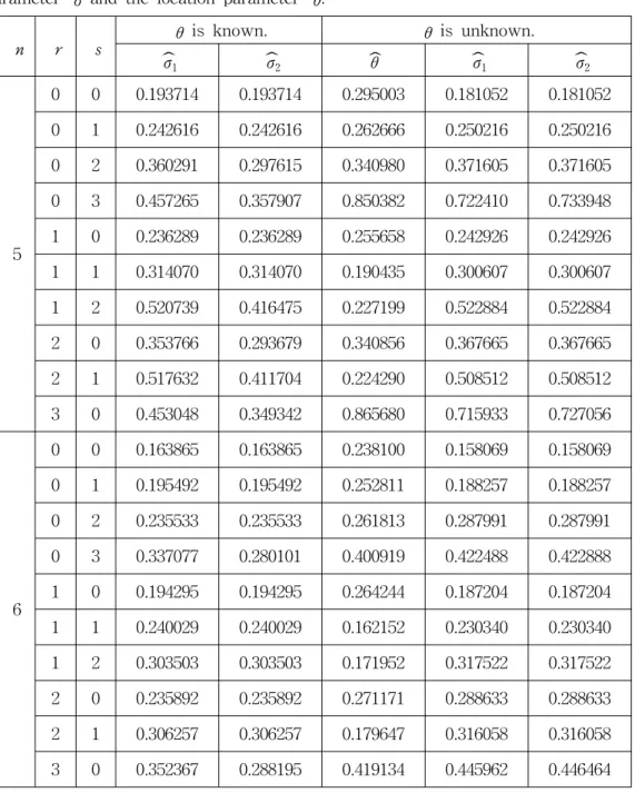
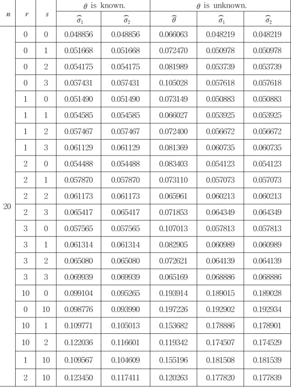
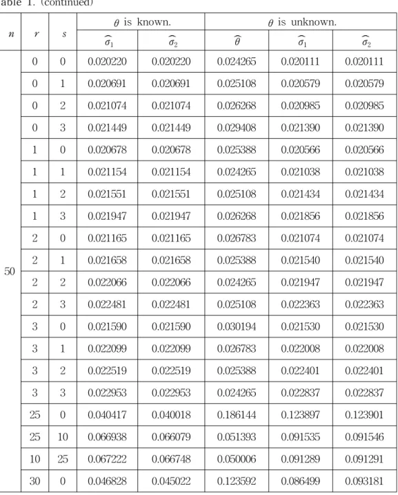
From the equations (2.11) and (2.14) in case 1, the equation (2.16) in case 2, the equations (2.20) and (2.23) in case 3, we simulate the mean squared errors of these two estimators of σ in the double exponential distribution for sample size n = 5, 6, 20, 50. The simulation procedure is repeated 10,000 times in Type-II censored samples. These values are given in Table 1. From Table 1, the estimator
σ2
ˆ is more efficient than ˆ in the sense of the mean squared error when the σ1 location parameter θ is known. But the estimator ˆ is more efficient than σ1 ˆ in σ2 the sense of the mean squared error when the location parameter θ is unknown.
The estimator ˆ is more simple than σ2 ˆ . The mean squared errors of all the σ1 estimators increase as r or s increases.
Table 1. The relative mean squared errors for the estimators of the scale parameter σ and the location parameter θ.
n r s
θ is known. θ is unknown.
σ1
ˆ σ
ˆ2 ˆθ σ
ˆ1 σ
ˆ2
5
0 0 0.193714 0.193714 0.295003 0.181052 0.181052
0 1 0.242616 0.242616 0.262666 0.250216 0.250216
0 2 0.360291 0.297615 0.340980 0.371605 0.371605
0 3 0.457265 0.357907 0.850382 0.722410 0.733948
1 0 0.236289 0.236289 0.255658 0.242926 0.242926
1 1 0.314070 0.314070 0.190435 0.300607 0.300607
1 2 0.520739 0.416475 0.227199 0.522884 0.522884
2 0 0.353766 0.293679 0.340856 0.367665 0.367665
2 1 0.517632 0.411704 0.224290 0.508512 0.508512
3 0 0.453048 0.349342 0.865680 0.715933 0.727056
6
0 0 0.163865 0.163865 0.238100 0.158069 0.158069
0 1 0.195492 0.195492 0.252811 0.188257 0.188257
0 2 0.235533 0.235533 0.261813 0.287991 0.287991
0 3 0.337077 0.280101 0.400919 0.422488 0.422888
1 0 0.194295 0.194295 0.264244 0.187204 0.187204
1 1 0.240029 0.240029 0.162152 0.230340 0.230340
1 2 0.303503 0.303503 0.171952 0.317522 0.317522
2 0 0.235892 0.235892 0.271171 0.288633 0.288633
2 1 0.306257 0.306257 0.179647 0.316058 0.316058
3 0 0.352367 0.288195 0.419134 0.445962 0.446464
Table 1. (continued)
n r s
θ is known. θ is unknown.
σ1
ˆ σ
ˆ2 ˆθ σ
ˆ1 σ
ˆ2
20
0 0 0.048856 0.048856 0.066063 0.048219 0.048219
0 1 0.051668 0.051668 0.072470 0.050978 0.050978
0 2 0.054175 0.054175 0.081989 0.053739 0.053739
0 3 0.057431 0.057431 0.105028 0.057618 0.057618
1 0 0.051490 0.051490 0.073149 0.050883 0.050883
1 1 0.054585 0.054585 0.066027 0.053925 0.053925
1 2 0.057467 0.057467 0.072400 0.056672 0.056672
1 3 0.061129 0.061129 0.081369 0.060735 0.060735
2 0 0.054488 0.054488 0.083403 0.054123 0.054123
2 1 0.057870 0.057870 0.073110 0.057073 0.057073
2 2 0.061173 0.061173 0.065961 0.060213 0.060213
2 3 0.065417 0.065417 0.071853 0.064349 0.064349
3 0 0.057565 0.057565 0.107013 0.057813 0.057813
3 1 0.061314 0.061314 0.082905 0.060989 0.060989
3 2 0.065080 0.065080 0.072621 0.064139 0.064139
3 3 0.069939 0.069939 0.065169 0.068886 0.068886
10 0 0.099104 0.095265 0.193914 0.189015 0.189028
0 10 0.098776 0.093990 0.197226 0.192902 0.192934
10 1 0.109771 0.105013 0.153682 0.178886 0.178901
10 2 0.122036 0.116601 0.119342 0.174507 0.174529
1 10 0.109567 0.104609 0.155196 0.181508 0.181539
2 10 0.123450 0.117411 0.120263 0.177820 0.177839
Table 1. (continued)
n r s
θ is known. θ is unknown.
σ1
ˆ σ
ˆ2 ˆθ σ
ˆ1 σ
ˆ2
50
0 0 0.020220 0.020220 0.024265 0.020111 0.020111
0 1 0.020691 0.020691 0.025108 0.020579 0.020579
0 2 0.021074 0.021074 0.026268 0.020985 0.020985
0 3 0.021449 0.021449 0.029408 0.021390 0.021390
1 0 0.020678 0.020678 0.025388 0.020566 0.020566
1 1 0.021154 0.021154 0.024265 0.021038 0.021038
1 2 0.021551 0.021551 0.025108 0.021434 0.021434
1 3 0.021947 0.021947 0.026268 0.021856 0.021856
2 0 0.021165 0.021165 0.026783 0.021074 0.021074
2 1 0.021658 0.021658 0.025388 0.021540 0.021540
2 2 0.022066 0.022066 0.024265 0.021947 0.021947
2 3 0.022481 0.022481 0.025108 0.022363 0.022363
3 0 0.021590 0.021590 0.030194 0.021530 0.021530
3 1 0.022099 0.022099 0.026783 0.022008 0.022008
3 2 0.022519 0.022519 0.025388 0.022401 0.022401
3 3 0.022953 0.022953 0.024265 0.022837 0.022837
25 0 0.040417 0.040018 0.186144 0.123897 0.123901
25 10 0.066938 0.066079 0.051393 0.091535 0.091546
10 25 0.067222 0.066748 0.050006 0.091289 0.091291
30 0 0.046828 0.045022 0.123592 0.086499 0.093181
References
1. Bain, L. J. and Engelhardt, M. (1973). Interval estimation for the two- parameter double exponential distribution, Technometrics, 15, 875-887.
2. Balakrishnan, N. (1989). Approximate MLE of the scale parameter of the Rayleigh distribution with censoring, IEEE Transactions on Reliability, 38, 355-357.
3. Balakrishnan, N. and Cutler, C. D. (1994). Maximum Likelihood Estimation of the Laplace parameters based on Type-II censored samples, In H. A. David Festschrift Volume (eds, D. F. Morrison, H. N.
Nagaraja, and P. K. Sen), New York: Springer-Verlag.
4. Childs, A. and Balakrishnan, N. (1996). Conditional inference procedures for the laplace distribution based on Type-II right censored samples, Statistics & Probability Letters, 31, 31-39.
5. Childs, A. and Balakrishnan, N. (2000). Conditional inference procedures for the laplace distribution when the observed samples are progressively censored, Metrika, 52, 253-265.
6. Govindarajulu, Z. (1966), Best linear estimates under symmetric
censoring of the parameters of a double exponential population, Journal of American Statistical Association, 61, 248-258.
7. Kang, S. B. (1996). Approximate MLE for the scale parameter of the double exponential distribution based on Type-II censored samples, Journal of the Korean Mathematical Society, 33, 69-79.
8. Kang, S. B., Suh, Y. S., and Cho, Y. S. (1997). Estimation of the parameters in an exponential distribution with Type-II censoring, The Korean Communications in Statistics, 4, 929-941.
9. Kappenman, R. F. (1975). Conditional confidence intervals for double exponential distribution parameters, Technometrics, 17, 233-235.
10. Raghunandanan K. and Srinivasan R. (1971). Simplified estimation of parameters in a double exponential distribution, Technometrics, 13, 689-691.
11. Shyu, J. C. and Owen, D. B. (1986a). One-sided tolerance intervals for the two-parameter double exponential distribution, Communications in Statistics- Simulation and Computation, 15, 101-119.
12. Shyu, J. C. and Owen, D. B. (1986b). Two-sided tolerance intervals for the two-parameter double exponential distribution, Communications in Statistics- Simulation and Computation, 15, 479-495.
[ received date : Oct. 2004, accepted date : Jan. 2005 ]