Estimation for the Half-Logistic Distribution Based on Multiply Type-II Censored Samples

Estimation for the Half-Logistic Distribution Based on Multiply Type-II Censored Samples

Suk-Bok Kang¹⁾ ․ Young Kou Park²⁾

Abstract

In this paper, we derive the approximate maximum likelihood estimators (AMLEs) of the scale parameter of the half-logistic distribution based on multiply Type-II censored samples. We compare the proposed estimators in the sense of the mean squared error (MSE) for various censored samples.

Keywords : Approximate maximum likelihood estimator, Half-Logistic distribution, Multiply Type-II censored sample

1. Introduction

A random variable _X is said to have a half-logistic distribution with the probability density function (pdf)

f ( x ; θ , σ ) =

2 exp

(

)

σ

{

(

)}

F ( x ; θ , σ ) =

1 - exp

(

)

1 + exp

(

)

1) First Author : Professor, Department of Statistics, Yeungnam University, Gyongsan, 712-749, Korea

E-mail : [email protected]

2) Associate Professor, Department of Mathematics, Yeungnam University, Gyongsan, 712-749,

E-mail : [email protected]

where _θ and _σ are the location and scale parameters, respectively.

The approximate maximum likelihood estimation method was first developed by Balakrishnan (1989) for the purpose of providing the explicit estimators of the scale parameter in the Rayleigh distribution. Kang (1996) obtained the AMLE for the scale parameter of the double exponential distribution based on Type-II censored samples and he showed that the proposed estimator is generally more efficient than the best linear unbiased estimator and the optimum unbiased absolute estimator.

Multiply Type-II censored sampling arises in a life-testing experiment whenever the experimenter does not observe the failure times of some units placed on a life-test. Another situation where multiply censored samples arise naturally is when some units failed between two points of observation with exact times of failure of these units unobserved.

Kong and Fei (1996) discussed the limit theorems for the maximum likelihood estimator under general multiply Type-II censoring. Recently, Kang (2003) proposed the AMLEs of the location and the scale parameters of the two-parameter exponential distribution with multiply Type-II censoring.

Application of the half-logistic distribution to life-testing had been well demonstrated by Balakrishnan (1985) who derived several recurrence relations satisfied by the single and the product moments of order statistics and applied them in a simple recursive process to compute the means, variances, and covariances of order statistics for sample sizes up to 15.

Balakrishnan and Joshi (1983) have obtained several recurrence relations for the moments and product moments of order statistics from a symmetrically truncated logistic distribution and applied them to tabulate the means, variances and covariances.

Balakrishnan and Puthenpura (1986) tabulated the coefficients of the best linear unbiased estimators of the location and scale parameters of the half-logistic distribution based on complete samples.

In this paper, we derive the AMLEs of the scale parameter _σ and the location parameter _θ based on multiply Type-II censored sample. We also compare the proposed estimators in the sense of the MSE for various censored samples.

2. Approximate Maximum Likelihood Estimators

Let us assume that the following multiply Type-II censored sample from a sample of size _n is

Xa1:n＜ X a2:n＜ … ＜ Xas:n (2.1) where _{1 ≤ a1＜ a2＜ … ＜ as≤ n}, and

a0= 0 , as + 1= n + 1 , F ( xa0:n) = 0 , F ( xas + 1:n) = 1 . (2.2) The likelihood function based on the multiply Type-II censored sample (2.1) can be written as

L = n!∏

s

j = 1f ( xaj:n)∏

s + 1 j = 1

[ F( x_aj:n) - F( x_{aj - 1:n})]^{aj- aj - 1- 1}

(aj- aj - 1- 1)! . (2.3)

The random variable _{Zi :n= ( Xi :n- θ ) / σ} has a standard half-logistic distribution with the pdf and cdf;

f ( z ) = 2e^{- z}

[1 +e^{- z}]^{2 , F ( z ) =}

1 -e^{- z}

1+e^{- z} , 0 ≤ z ＜ ∞.

The _{f ( z)}, _{f '( z),} and _{F ( z)} satisfy as f '( z) = - F ( z) f ( z) f ( z) = [ 1 - F ( z)] [ 1 + F ( z)] / 2 .

From the equation (2.3), the likelihood function is a monotonically increasing function of _θ. Thus the MLE of _θ is ^ˆ_{θ = Xa}

1:n.

On differentiating the log-likelihood function with respect to _σ in turn and equation to zero, we obtain the estimating equation as

∂ ln L

∂σ = - 1

2 σ

[

- ( n - as) Zas:n-(n-as) F( Zas:n) Zas:n-2∑

s

j = 1F( Zaj:n) Zaj:n

+ 2∑^s

j = 2(aj-aj - 1-1) f( Zaj:n)Zaj:n- f( Zaj - 1:n)Zaj - 1:n

F( Zaj:n) - F( Zaj - 1:n)

]

(2.4)

Since the likelihood equation is very complicated, the equation (2.4) does not admit an explicit solution for _σ.

Let

ξ_i= F^{- 1}(p_i) =- ln

(

)

We may approximate the following functions in Taylor series around the points ξa1, ξas, ξaj, and _{( ξa}

j, ξaj - 1), respectively.

f( Za1:n)

F( Za1:n) ≃ α11+ β11Za1:n (2.5)

F( Za_j:n) Za_j:n≃ δ1j+ κ1jZ a_j:n (2.6)

f( Zaj:n)Zaj:n- f( Zaj - 1:n)Zaj - 1:n

F( Z_aj:n) - F( Z_{aj - 1:n}) ≃ α_j+ β_jZ_aj:n+ γ_jZ_{aj - 1:n} (2.7)

1

F( Za₁:n) ≃ α₂₁+ β₂₁Z_a1:n (2.8)

F( Zaj:n) ≃ δ2j+ κ2jZaj:n (2.9)

f( Z_aj:n)

F( Zaj:n) - F( Zaj - 1:n) ≃ α1j+ β1jZa_j:n+ γ1jZ a_{j - 1}:n (2.10)

f( Zaj - 1:n)

F( Z_aj:n) - F( Z_{aj - 1:n}) ≃ α_2j+ β_2jZ_aj:n+ γ_2jZ _{aj - 1:n} (2.11) where

α11= f ( ξa1)

[

]

β11= 1

pa1

[

]

δ1j= - f( ξaj)ξaj

2

κ1j= f ( ξaj) ξaj+ paj

α_j= ξ_aj²f ( ξ_aj) p_aj- ξ_{aj - 1}²f ( ξ_{aj - 1}) p_{aj - 1}

p_aj-p_{aj - 1} +

[

]

βj= f( ξaj)

paj- paj - 1

[

]

γj= - f( ξ_{aj - 1})

paj- paj - 1

[

]

α21= 1

pa1

[

]

β₂₁= - f ( ξa1) p_a1²

δ2j= paj- f ( ξaj) ξaj

κ2j= f( ξaj)

α1j= f( ξaj)

p_aj- p_{aj - 1}

[

]

β1j= - f ( ξaj)

paj- paj - 1

[

]

γ1j= f( ξ_aj)f( ξ_{aj - 1}) [ paj- paj - 1]²

α2j= f( ξ_{aj - 1})

paj- paj - 1

[

]

β_2j= - f( ξ_aj)f( ξ_{aj - 1})

[ paj- paj - 1]² = - γ_1j

γ_2j= - f ( ξaj - 1)

p_aj- p_{aj - 1}

[

]

By substituting the equations (2.5), (2.6), and (2.7), into the equation (2.4), we can derive an estimator of _σ as follows;

σ₁

ˆ₌ ^{B1+ C1ˆθ}

A₁ (2.12)

where

A₁= 2 s +( a₁-1) ( α₁₁- δ₁₁) - ( n - a_s) δ_1s-2∑

s

j = 1δ_1j+ 2∑

s

j = 2(a_j-a_{j - 1}-1)α_j

B1 = ( a1-1) ( κ11-β11) Xa1:n-( n - as) ( 1 +κ1s) Xas:n-2∑^s

j = 1κ1jXaj:n

-2∑

s

j = 2(a_j-a_{j - 1}-1)( β_jX_aj:n+γ_jX_{aj - 1:n})

C1= ( a1-1) ( β11- κ11) - ( n - as) ( 1 + κ1s) - 2∑^s

j = 1κ1j+ 2∑^s

j = 2(aj-aj - 1-1)( βj+ γj) . By substituting the equations (2.7), (2.8), and (2.9), into the equation (2.4), we can derive an estimator of _σ as follows;

σ2

ˆ₌ ^{- B2+ B22+ 4 A2C2} 2 A2

(2.13)

where

A2= 2

[

]

B₂ = ( a₁-1) ( α₂₁- δ₂₁) X_a1:n- ( n - a_s) ( 1 +δ_2s) X_as:n- 2∑

s

j = 1δ_2jX_aj:n

_{+ 2}∑^s

j = 2(aj- aj - 1-1)( βjXaj:n+ γjXaj - 1:n) _-

[

j = 1δ2j+ 2∑^s

j = 2(aj-aj - 1-1)( βj+ γj)

]

C2= ( a1-1) ( β21- κ21) ( X a1:n- θˆ₎²_{- ( n - a}

s) κ2s( Xas:n- θˆ₎²_{- 2}∑^s

j = 1κ2j( Xaj:n- θˆ₎²_. By substituting the equations (2.5), (2.6), (2.10), and (2.11) into the equation (2.4), we can derive an estimator of _σ as follows;

σ3

ˆ₌ ^{- B3+ B32+ 4 A3C3} 2 A3

(2.14)

where

A3= 2 s + ( a1-1) ( α11- δ11)-(n-as) - 2∑

s j = 2δ1j

B₃= ( a₁-1) ( β₁₁- κ₁₁) X_a1:n- ( n - a_s) ( 1 + κ_1s) X_as:n- 2∑^s

j = 1κ_1jX_aj:n +2∑

s

j = 2(aj-aj - 1-1)( α1jXa_j:n-α2jXa_{j - 1}:n) -

[

s

j = 1κ1j+ 2∑

s

j = 2(aj-aj - 1-1)( α1j- α2j)

]

C₃ = 2∑

s

j = 1(a_j- a_{j - 1}-1){^{β1j( Xa}j:n- θˆ₎²_{+2 γ}

1j( X _aj:n- θˆ_{) ( X}

aj - 1:n- θˆ₎ - γ2j( Xaj - 1:n- θˆ₎²}^.

By substituting the equations (2.8), (2.9), (2.10), and (2.11) into the equation (2.4), we can derive an estimator of _σ as follows;

σ4

ˆ₌ ^{- B4+ B42+ 8 s C4}

4 s (2.15)

where

B4= ( a1-1) ( α21- δ21) Xa1:n- ( n - as) ( 1 + δ2s) Xas:n- 2∑

s

j = 1δ2jXaj:n

+2∑^s

j = 2(aj-aj - 1-1)( α1jXaj:n-α2jXaj - 1:n) -

[

j = 1δ_2j+ 2∑^s

j = 2(a_j-a_{j - 1}-1)( α_1j- α_2j)

]

C4= C2+ C3.

For the half-logistic distribution the maximum likelihood method does not provide an explicit estimator for the scale parameter based on either complete or multiply Type-II censored samples. But we provided several explicit estimators by approximating the likelihood function.

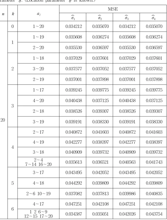
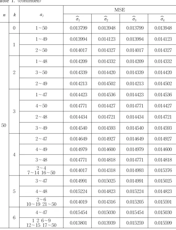
From the equations (2.12) to (2.15), the MSEs of these estimators are simulated by Monte Carlo method for sample size _{n = 20, 50} and various choices of censoring. These values are given in Table 1.

From Table 1, the estimators ˆ and _σ2 ˆ are generally more efficient than _σ4 ˆ _σ1 and ˆ in the sense of the MSE. But _σ3 ˆ is simpler than the other estimators.σ₁

References

1. Balakrishnan, N. (1985). Order statistics from the half logistic distribution. Journal of Statistical Computation and Simulation, 20, 287-309.

2. Balakrishnan, N. (1989). Approximate MLE of the scale parameter of the Rayleigh distribution with censoring, IEEE Transactions on Reliability, 38, 355-357.

3. Balakrishnan, N. and Joshi, P. C. (1983). Single and product moments of order statistics from symmetrically truncated logistic distribution.

Demonstratio Mathematica, 16, 833-841.

4. Balakrishnan, N. and Puthenpura, S. (1986). Best linear unbiased estimators of location and scale parameters of the half logistic distribution. Journal of Statistical Computation and Simulation, 25, 193-204.

5. Kang, S. B. (1996). Approximate MLE for the scale parameter of the double exponential distribution based on Type-II censored samples, Journal of the Korean Mathematical Society, 33, 69-79.

6. Kang, S. B. (2003). Approximate MLEs for exponential distribution under multiple Type-II censoring, Journal of the Korean Data & Information Science Society, 14, 983-988.

7. Kong, F. and Fei, H. (1996). Limit theorems for the maximum likelihood estimate under general multiply Type-II censoring, Annals of the

Institute of Statistical Mathematics, 48, 731-755.

Table 1. The relative mean squared errors for the estimators of the scale parameter _σ. (Location parameter _θ is known.)

n k aj

MSE σ₁

ˆ _σ

ˆ2 _σ

ˆ3 _σ

ˆ4

20

0 1∼20 0.034212 0.035070 0.034212 0.035070

1

1∼19 0.035608 0.036274 0.035608 0.036274 2∼20 0.035530 0.036597 0.035530 0.036597

2

1∼18 0.037029 0.037601 0.037029 0.037601 3∼20 0.037577 0.037052 0.037577 0.037052 2∼19 0.037001 0.037898 0.037001 0.037898

3

1∼17 0.039245 0.039775 0.039245 0.039775 4∼20 0.040438 0.037125 0.040438 0.037125 2∼18 0.038526 0.039307 0.038526 0.039307 3∼19 0.039191 0.038330 0.039191 0.038330

4

2∼17 0.040872 0.041603 0.040872 0.041603 4∼19 0.042277 0.038397 0.042277 0.038397 3∼18 0.040909 0.039732 0.040909 0.039732

2∼4

7∼14 16∼20 0.035613 0.036521 0.040563 0.041743

5

3∼17 0.043495 0.042052 0.043495 0.042052 4∼18 0.044292 0.039809 0.044292 0.039809 2∼6 10∼19 0.037082 0.037813 0.039986 0.040835

6

4∼17 0.047251 0.042108 0.047251 0.042108 1 2 6∼9

12∼15 17∼20 0.034387 0.035051 0.042026 0.043754

Table 1. (continued)

n k aj

MSE σ1

ˆ _σ

ˆ2 _σ

ˆ3 _σ

ˆ4

50

0 1∼50 0.013799 0.013948 0.013799 0.013948

1

1∼49 0.013994 0.014123 0.013994 0.014123 2∼50 0.014017 0.014327 0.014017 0.014327

2

1∼48 0.014209 0.014332 0.014209 0.014332 3∼50 0.014339 0.014420 0.014339 0.014420 2∼49 0.014213 0.014502 0.014213 0.014502

3

1∼47 0.014423 0.014536 0.014423 0.014536 4∼50 0.014771 0.014427 0.014771 0.014427 2∼48 0.014434 0.014721 0.014434 0.014721 3∼49 0.014540 0.014593 0.014540 0.014593

4

2∼47 0.014649 0.014927 0.014649 0.014927 4∼49 0.014979 0.014600 0.014979 0.014600 3∼48 0.014771 0.014818 0.014771 0.014818

2∼4

7∼14 16∼50 0.014017 0.014318 0.014993 0.015376

5

3∼47 0.014991 0.015025 0.014991 0.015025 4∼48 0.015224 0.014823 0.015224 0.014823

2∼6

10∼19 21∼50 0.014019 0.014316 0.015205 0.015591 6

4∼47 0.015454 0.015030 0.015454 0.015030 1 2 6∼9

12∼15 17∼50 0.013801 0.013939 0.015259 0.015599

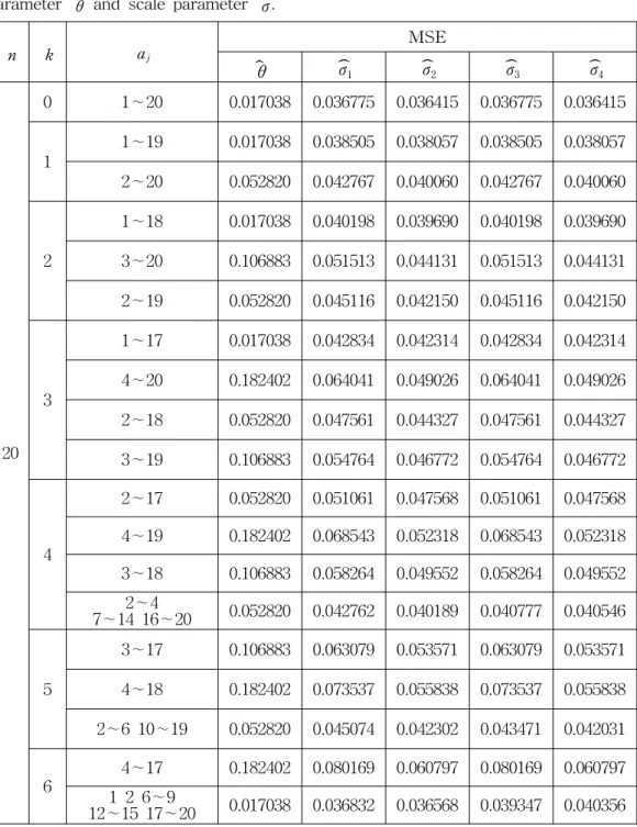
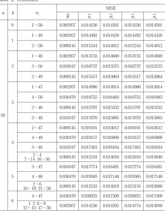
Table 2. The relative mean squared errors for the estimators of the location parameter _θ and scale parameter _σ.

n k aj

MSE

ˆθ ˆ_{σ1 σ}

ˆ2 _σ

ˆ3 _σ

ˆ4

20

0 1∼20 0.017038 0.036775 0.036415 0.036775 0.036415

1

1∼19 0.017038 0.038505 0.038057 0.038505 0.038057 2∼20 0.052820 0.042767 0.040060 0.042767 0.040060

2

1∼18 0.017038 0.040198 0.039690 0.040198 0.039690 3∼20 0.106883 0.051513 0.044131 0.051513 0.044131 2∼19 0.052820 0.045116 0.042150 0.045116 0.042150

3

1∼17 0.017038 0.042834 0.042314 0.042834 0.042314 4∼20 0.182402 0.064041 0.049026 0.064041 0.049026 2∼18 0.052820 0.047561 0.044327 0.047561 0.044327 3∼19 0.106883 0.054764 0.046772 0.054764 0.046772

4

2∼17 0.052820 0.051061 0.047568 0.051061 0.047568 4∼19 0.182402 0.068543 0.052318 0.068543 0.052318 3∼18 0.106883 0.058264 0.049552 0.058264 0.049552

2∼4

7∼14 16∼20 0.052820 0.042762 0.040189 0.040777 0.040546

5

3∼17 0.106883 0.063079 0.053571 0.063079 0.053571 4∼18 0.182402 0.073537 0.055838 0.073537 0.055838 2∼6 10∼19 0.052820 0.045074 0.042302 0.043471 0.042031

6

4∼17 0.182402 0.080169 0.060797 0.080169 0.060797 1 2 6∼9

12∼15 17∼20 0.017038 0.036832 0.036568 0.039347 0.040356

Table 2. (continued)

n k aj

MSE ˆθ _σ

ˆ1 _σ

ˆ2 _σ

ˆ3 _σ

ˆ4

50

0 1∼50 0.002957 0.014256 0.014201 0.014256 0.014201

1

1∼49 0.002957 0.014492 0.014428 0.014492 0.014428 2∼50 0.009145 0.015244 0.014812 0.015244 0.014812

2

1∼48 0.002957 0.014735 0.014669 0.014735 0.014669 3∼50 0.018347 0.016737 0.015575 0.016737 0.015575 2∼49 0.009145 0.015517 0.015064 0.015517 0.015064

3

1∼47 0.002957 0.014986 0.014914 0.014986 0.014914 4∼50 0.030479 0.018755 0.016483 0.018755 0.016483 2∼48 0.009145 0.015797 0.015332 0.015797 0.015332 3∼49 0.018347 0.017070 0.015865 0.017070 0.015865

4

2∼47 0.009145 0.016101 0.015612 0.016101 0.015612 4∼49 0.030479 0.019157 0.016808 0.019157 0.016808 3∼48 0.018347 0.017403 0.016164 0.017403 0.016164

2∼4

7∼14 16∼50 0.009145 0.015243 0.014816 0.015010 0.014940

5

3∼47 0.018347 0.017774 0.016481 0.017774 0.016481 4∼48 0.030479 0.019565 0.017148 0.019565 0.017148

2∼6

10∼19 21∼50 0.009145 0.015243 0.014819 0.015116 0.015080 6

4∼47 0.030479 0.020025 0.017509 0.020025 0.017509 1 2 6∼9

12∼15 17∼50 0.002957 0.014256 0.014205 0.014774 0.014938

[ received date : Nov. 2004, accepted date : Jan. 2005 ]