Genetic Diversity of Common Reed in Korea Based on Morphological Characteristics and Random Amplified Polymorphic DNA Markers
Hyosub Chu1, Won Kyong Cho2*, Yeonggil Rim3, Yeonhwa Jo3 and Jae-Yean Kim3*
1Bioindustrial Process Center, Jeonbuk Branch Institute of Korea Research Institute of Bioscience and Biotechnology (KRIBB), Jeongeup 580-185, Korea
2Department of Agricultural Biotechnology, Seoul National University, Seoul 151-921, Korea
3Division of Applied Life Science (BK21 program), Environmental Biotechnology National Core Research Center, PMBBRC, Gyeongsang National University, Jinju 660-701, Korea
Abstract - To elucidate genetic diversity of common reed in Korea, we collected a total of 674 common reed plants from 27 regions in South Korea. Hierarchical clustering using 7 morphological traits divided the 27 common reed populations into 7 groups. Random amplified polymorphic DNA (RAPD) results identified three distinct groups of common reed. Common reed accessions in group I mostly inhabit coastal areas. Group II includes reeds mostly collected from inland areas. Group III consists of common reed accessions collected from inland and coastal areas, suggesting that this group might contain hybrids. In summary, we suggest that parapatric speciation might be an important factor in the genetic diversity of common reed and geographical speciation of common reed that might be also affected by environmental gradients.
Key words - Marker, Morphology, RAPD, Reed, Variation
*Corresponding author. E-mail : [email protected], [email protected]
Introduction
Common reed (Phragmites australis) is a tall, perennial grass growing to 16 feet or more in height. This plant can be found almost everywhere, ranging from the tropics to cold- temperate regions around the world, and it grows mainly in wetlands, such as coastal regions and lakeshores (Brix, 1999;
Engloner, 2009; Kim et al., 2009). Common reed can propagate both by seeds and by vegetative spread through pieces of rhizome (League et al., 2006). Because of its vigorous growth characteristic, common reed is regarded as an invasive plant that can destruct ecosystems by expelling native plants after it is introduced into new marsh communities (Chun and Choi, 2009). As a result, the marsh hydrology and wildlife habitat can be changed with a high possibility for fires (Meyerson et al., 2000).
In spite of the ecological problem, this common reed has significant ecological merits (Kozłowska et al., 2009; Peruzzi et al., 2009). For example, it diminishes contamination of
waste water produced from industry, agriculture and private residences and is also essential for wildlife and conservation, especially in Asia and Europe (Cui et al., 2009; Kozłowska et al., 2009). Furthermore, the reed has been traditionally used as a material for making mats, boater hats, furniture, baskets and handicrafts (Dogan et al., 2008). Genetic diversity of various common reed in the world has been studied using several molecular markers including AFLP, RAPD (Lambertini et al., 2006; Lambertini et al., 2008; Oh et al., 2006) and RFLP (Saltonstall, 2003).
In order to investigate the genetic diversity and certain factors affect the morphological traits of common reed, we collected a total of 674 common reed plants from 27 regions in Korea and determined their morphological and genetic diversity by RAPD markers.
Materials and Methods
Collection of common reed
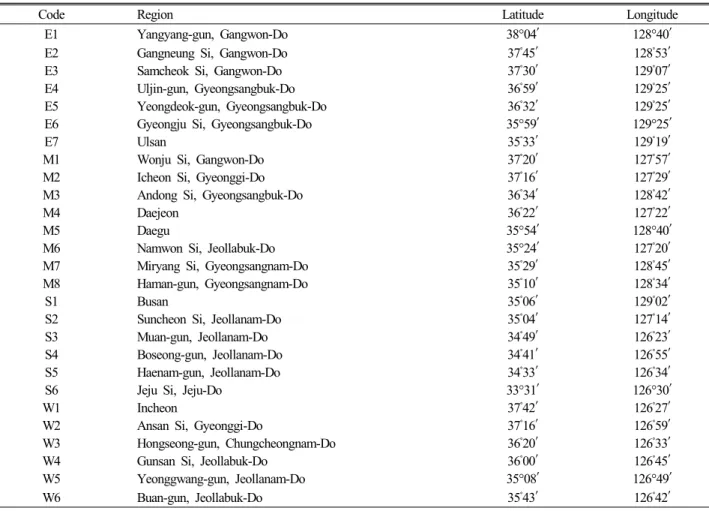
We collected a total of 674 common reed plants from 27 regions of South Korea (Fig. 1). Detailed information on the sampling regions is available in Table 1. The samples were
Table 1. Detailed information for sampling regions of common reed in Korea.
Code Region Latitude Longitude
E1 Yangyang-gun, Gangwon-Do 38°04′ 128°40′
E2 Gangneung Si, Gangwon-Do 37˚45′ 128˚53′
E3 Samcheok Si, Gangwon-Do 37˚30′ 129˚07′
E4 Uljin-gun, Gyeongsangbuk-Do 36˚59′ 129˚25′
E5 Yeongdeok-gun, Gyeongsangbuk-Do 36˚32′ 129˚25′
E6 Gyeongju Si, Gyeongsangbuk-Do 35°59′ 129°25′
E7 Ulsan 35˚33′ 129˚19′
M1 Wonju Si, Gangwon-Do 37˚20′ 127˚57′
M2 Icheon Si, Gyeonggi-Do 37˚16′ 127˚29′
M3 Andong Si, Gyeongsangbuk-Do 36˚34′ 128˚42′
M4 Daejeon 36˚22′ 127˚22′
M5 Daegu 35°54′ 128°40′
M6 Namwon Si, Jeollabuk-Do 35°24′ 127˚20′
M7 Miryang Si, Gyeongsangnam-Do 35˚29′ 128˚45′
M8 Haman-gun, Gyeongsangnam-Do 35˚10′ 128˚34′
S1 Busan 35˚06′ 129˚02′
S2 Suncheon Si, Jeollanam-Do 35˚04′ 127˚14′
S3 Muan-gun, Jeollanam-Do 34˚49′ 126˚23′
S4 Boseong-gun, Jeollanam-Do 34˚41′ 126˚55′
S5 Haenam-gun, Jeollanam-Do 34˚33′ 126˚34′
S6 Jeju Si, Jeju-Do 33°31′ 126°30′
W1 Incheon 37˚42′ 126˚27′
W2 Ansan Si, Gyeonggi-Do 37˚16′ 126˚59′
W3 Hongseong-gun, Chungcheongnam-Do 36˚20′ 126˚33′
W4 Gunsan Si, Jeollabuk-Do 36˚00′ 126˚45′
W5 Yeonggwang-gun, Jeollanam-Do 35°08′ 126°49′
W6 Buan-gun, Jeollabuk-Do 35˚43′ 126˚42′
The code, regional name latitude and longitude for each common reed population are described.
Fig. 1. A map of South Korea showing the 27 sampling regions.
The individual code indicates the region of sampling. Each code was based on a direction and latitude, like seven regions in the eastern part of the country (named E1 to E7), eight inland regions (from M1 to M8), six southern regions (from S1 to S6) and six western regions (from W1 to W6). Detailed information for the sampling regions is listed in Table 1.
collected in November 2008. A majority of the sampling regions are located along the coast.
Measurement of morphological characteristics
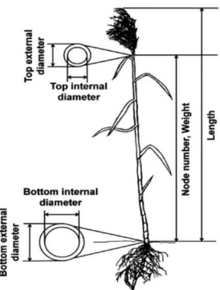
In November 2008, at the end of the growing season, the shoot length, number of nodes, bottom outer diameter, bottom inner diameter, top outer diameter, top inner diameter and dry weight for each collected reed were determined. Detailed information for morphological characteristics was drawn in Fig. 2.
Genomic DNA isolation
For Random Amplified Polymorphism DNA (RAPD) analysis, we selected one representative sample from each common reed population resulting in 28 accessions. Harvested leaf materials were immediately frozen in liquid nitrogen and were kept at -80℃. Total genomic DNA was prepared
Fig. 2. Illustration of seven morphological traits of P. australis.
All collected P. australis were analyzed based on seven morphological traits: shoot length, number of nodes, bottom outer diameter, bottom inner diameter, top outer diameter, top inner diameter and dry weight.
using a DNeasy® Plant Mini Kit (QIAGEN GmbH, Hilden, Germany) according to the manufacturer’s instructions.
RAPD analysis
For RAPD experiments, a set of random primers was obtained from Operon’s RAPD 10 mer Kits (Operon Technologies, Inc., Alameda, CA.). A total of 20 random primers (OPC1-OPC20) were tested. Among them, OPC1, 2, 5, 18, 19 and OPC20 were selected for RAPD analysis. The PCR mixture used contained genomic DNA, diluted to a final concentration of 2 ng/μl, 0.1 μl (10 mM dNTP mix), 2 μl of 10-mer random primer (10 pmole/μl), 0.5 μl of Taq DNA polymerase (2.5 Units/μl), 2 μl of 10X Taq buffer (SolGent Co., Ltd., Daejeon, South Korea) and distilled water to a final volume of 20 μl.
PCR for RAPD analysis was performed in a MJ Research- Peltier Thermal Cycler PTC-200 programmed for an initial step of 4 min at 94℃, then 40 repeats of 30 s at 94℃, 60 s at 35℃ and 2 min at 72℃ followed by a final termination step of 5 min at 72℃. RAPD experiments were repeated three times and amplified major DNA fragments were selected for statistical analysis using Excel (Microsoft Excel 2007, Redmond, USA).
Statistical analyses
Statistical Package for the Social Sciences (SPSS) was used
for the statistical analysis (One-way analysis of variation).
For the use of RAPD results in the MEGA4 program, the data was converted as follows: the presence of a fragment was noted by a T, whereas its absence was noted by an A. A phylogenetic tree was created using the MEGA4 program with the UPGMA method.
Hierarchical clustering
To divide common reed populations based on morphological traits, each obtained value was normalized by 7 morphological traits and 27 populations. Normalized values were subjected to hierarchical clustering using the Genesis program (Sturn et al., 2002).
Results
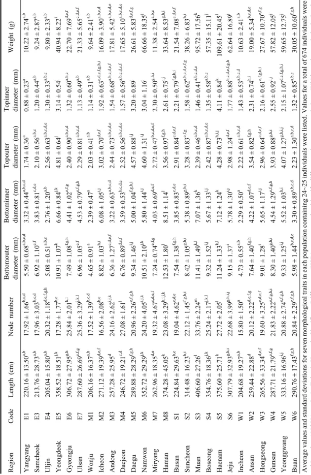
Morphological characteristics of Korean Phragmites australis The S3 population had the greatest length and number of nodes, the M8 population had the largest bottom inner and outer diameters, the E5 population had the largest top inner diameter and the S5 population had the largest top outer diameter and the highest weight, according to the analysis of morphological traits (Table 2). Interestingly, it was very difficult to find correlations among the morphological traits.
For instance, the S3 population was the tallest and had the highest number of nodes, but its other traits did not have as high values as those of other populations.
For each morphological trait, the 27 populations could be divided into 11 to 13 different subgroups (Table 1). For example, the E2, S3 and S5 populations belong to only one subgroup based on length, node number and weight. The E7 and M7 populations belong to at least two subgroups based on all traits. Based on node number, top outer diameter and top inner diameter, a majority of populations belonged to several subgroups with a maximum of seven groups (Table 1). As a result, morphological traits of common reed could not distinguish all 27 populations clearly. Therefore, we performed hierarchical clustering as an alternative. Hierarchical clustering based on morphological traits identified seven subgroups of common reed (Fig. 3). For example, group A, which includes the S2, E1, S3, S4 and S6 populations, has relatively higher values for five of the morphological traits
Fig. 3. Hierarchical clustering to group 27 common reed populations based on the 7 morphological traits. For the hierarchical clustering, average values for the 7 morphological traits in the 27 populations were used. First, values were normalized twice by 7 morphological traits and 27 populations.
Using the complete linkage method with the default parameters implemented in the Genesis program, 7 morphological traits and 27 common reed populations were hierarchically clustered.
Black and white indicate relatively high and low values, respectively. The seven clustered groups are indicated by bars (Group A to G). Abbreviations used for the seven morphological traits are: ‘W’ Weight, ‘NN’ Node number, ‘BOD’ Bottom outer diameter, ‘BID’ Bottom inner diameter, ‘L’ Length,
‘TOD’ Top outer diameter and ‘TID’ Top inner diameter.
Fig. 4. Electrophoresis image of RAPD results. Amplified PCR products were separated on 1.5% agarose gels in 0.5X TBE buffer with two lanes of 1 Kb DNA ladder (SolGent Co., Ltd., Daejeon, South Korea) and three lanes for out-groups (Phragmites japonica, Arabidopsis thaliana and Oryza sativa).
A total of 129 RAPD polymorphisms were detected from the six primers (OPC1, 2, 5, 18, 19 and OPC20).
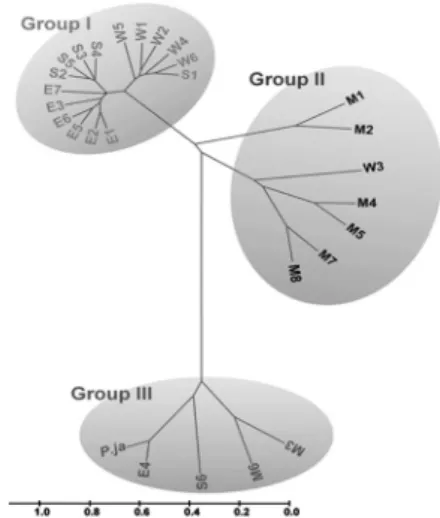
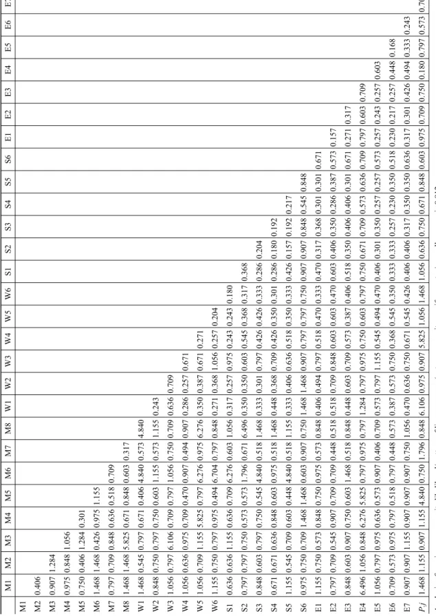
Fig. 5. A phylogenetic tree based on RAPD results identified three different groups of common reed. The 27 common reed accessions were divided into 3 distinct groups (Groups I, II and III). The scale bar indicates genetic distances.
(all except the top outer and inner diameters) than other populations. The group C showed a totally opposite pattern compared to those in group A. Moreover, group G, containing five populations, had the highest values only for the number of nodes (Fig. 3).
Previously, it has been shown that the amount of solar radiation is an important environmental factor that promotes growth of P. australis (Charles-Edwards, 1982). Normally, the amount of solar radiation is dependent on latitude. To test for a correlation between the amount of solar radiation and the length of plants, information for the amount of solar radiation (from December 2007 to November 2008) at each location was obtained from the Korea Meteorological Administration (http://www.kma.go.kr). Unexpectedly, we could not find a correlation between the length of common reed plants and the amount of solar radiation (data not shown).
RAPD analysis
Molecular markers have been powerful tools to analyze genetic divergence of various plant species. Among them, RAPD is the simplest and least expensive technique for detecting polymorphisms using arbitrary primers (Kim et al., 2009; Lambertini et al., 2008). To investigate the genetic diversity of common reed, we performed RAPD analysis. We selected 6 primers amplifying a total of 129 polymorphic bands from 28 accessions (Fig. 4). Using RAPD results, we
analyzed pairwise distances and created phylogenetic tree for 28 accessions of common reeds (Table 3). In the phylogenetic tree based on the identified polymorphisms, common reed are divided into three distinct groups (Groups I, II and III) (Fig.
5). Group I contains mostly collected from coastal regions or near river mouths, whereas group III includes the S6, M6, M3 and E4 accessions as well as P. japonica as a control. Group II covers P. australis derived from inlands or middle rivers.
This data supports the idea that genetic characteristics of common reeds are closely related to environmental factors that are often caused by geographical locations.
The results of the RAPD analysis showed that the common reeds seem to be diverged according to their geographical locations, such as coastal areas (Group I) and riversides (Group II). Group III identified by the RAPD analysis contains accessions of common reed growing in inland areas, such as M3 and M6, the S6 (Jeju island) accession, the coastal E4 accession and P. japonica.
Discussion
Characteristics of the representative common reed RAPD results identified three distinct groups of common reed that might be good examples to explain the speciation of Korean P. australis. The representative features of common reed might be those of the common reed accessions in group I based on their natural habitats of mostly coastal areas.
Moreover, P. australis in group I might be more tolerant of salinity than common reed. This salt-tolerance is caused by the unusual geographical feature of South Korea that it is surrounded by seas.
Geographical speciation of common reed
Group II from the RAPD analysis includes common reed mostly collected from inland areas, such as riversides. They might have originated from P. australis adapted to coastal regions that gradually expanded inland, inhabiting areas near rivers. Moreover, accessions in group II could not be detected in eastern areas, in which the area inhabited by common reed is physically restricted by geographical barriers, such as the Taebaek Ridge Mountains. This mountain range runs along the East Sea from Hwangnyong Mountain in North Korea to
Busan in South Korea. In contrast, the mountain ranges of the western and southern regions of South Korea are gentler than those of the east. Thus, the biggest two rivers of South Korea, the Han and the Nakdong, can stretch to the southwest. We propose that common reed inhabiting coastal areas could expand inland along with rivers. Similarly, the previous study has shown ecological role of mountain ridges to conserve biodiversity within restricted area in Korea (Cho et al., 2008).
As a result, populations of group II in different environmental conditions, such as fresh water, can be explained by parapatric speciation. Parapatric speciation refers to organisms that are separated by environmental conditions (Antonovics, 1971;
Caisse and Antonovics, 1978; Doebeli and Dieckmann, 2003).
Group III in the RAPD analysis includes common reed populations collected from inland and coastal areas. Interestingly, some P. australis populations belong to group III with P.
japonica based on RAPD analysis. These data indicate that these P. australis, along with P. japonica, might have similar genetic characteristics with which they might adapt well to certain environmental conditions.
Morphological diversity of Korean P. australis
Although we divided the 27 P. australis populations into 7 groups based on morphological traits, it was hard to explain their diversity by molecular markers. Numerous studies have shown that several factors can influence the morphology of common reed species. For instance, radiation, geographical location, salinity, biotic attacks and ploidy level can affect growth of P. australis (Brix, 1999; Hansen et al., 2007).
Previous studies suggested that ploidy level might play an important role in determining the morphologies of P.
australis. P. australis is known to be an allopolyploid with a wide range of euploidy levels (Raicu et al., 1972). Among them, tetraploids (2n = 48) and octoploids (2n = 96) are commonly found (Clevering and Lissner, 1999). In general, octoploids had larger leaves, shoots and cells than hexaploids and tetraploids (Paucã-Comãnescu et al., 1999).
Pollen fertility or sterility was also caused by ploidy levels.
For example, hexaploids tend to be sterile, unlike plants with other ploidy levels, as shown in previous studies (Björk, 1967; Gorenflot et al., 1990). Despite the lack of information related to the ploidy level of Korean P. australis, we found
that common reed in the M4 population did not have seeds, suggesting that this population might be hexaploid. Thus, we suppose that Korean P. australis is composed of various polyploids.
Although we attempted to use genetic markers to explain the diverse morphological traits of common reed, but there was not enough data from genetic markers to explain the morphological diversity, suggesting that additional experimental approaches, such as investigation of the ploidy level, should be performed. Similarly, morphological characteristics and RAPD markers have been used to reveal genetic diversity of Korean Calanthe (Cho et al., 2010). Thus, combination of phenotypes and molecular markers could be a useful tool for plant genetic diversity.
In this study, we studied genetic diversity of common reed based on morphological traits and RAPD markers. The results suggest that the various morphological traits of P. australis populations in Korea are caused by parapatric speciation.
Furthermore, our results explain geographical speciation of common reed that might be also affected by environmental gradients.
Acknowledgement
This work was supported by the National Research Foundation of Korea (NRF) grant funded by the Korea government (MEST) (No. 2011-0010027) and a grant from the Next-Generation BioGreen 21 Program (No. PJ00798402), Rural Development Administration, Republic of Korea.
Literature Cited
Antonovics, J. 1971. The effects of a heterogeneous environment on the genetics of natural populations. American Sci. 59:
593-599.
Björk, S. 1967. Ecologic investigations of Phragmites communis.
Studies in theoretic and applied limnology. Folia Limnol.
Scand. 14:1-248.
Brix, H. 1999. Genetic diversity, ecophysiology and growth dynamics of reed (Phragmites australis). Aquat. Bot. 64:
179-184.
Caisse, M. and J. Antonovics. 1978. Evolution in closely
adjacent plant populations. IX. Evolution of reproductive isolation in clinal populations. Heredity 40:371-384.
Charles-Edwards, D.A. 1982. Physiological Determinants of Crop Growth, Academic Press, Sydney, Australia. pp. 1-161.
Cho, D.H., M.Y. Chung, S.O. Jee, C.K. Kim, J.D. Chung and K.M. Kim. 2010. Intraspecific morphological characteristics and genetic diversity of Korean Calanthe. Korean J. Plant Res. 23:541-549.
Cho, K.H., SK. Hong and DS. Cho. 2008. Ecological role of mountain ridges in and around Gwangneung royal tomb forest in central Korea. J. Plant Biol. 51:387-394.
Chun, YM. and Y.D. Choi. 2009. Expansion of Phragmites australis (Cav.) Trin. ex Steud. (common reed) into Typha spp. (cattail) wetlands in northwestern Indiana, USA. J. Plant Biol. 52:220-228.
Clevering, O.A. and J. Lissner. 1999. Taxonomy, chromosome numbers, clonal diversity and population dynamics of Phragmites australis. Aquat. Bot. 64:185-208.
Cui, B., Q. Yang, Z. Yang and K. Zhang. 2009. Evaluating the ecological performance of wetland restoration in the Yellow River Delta, China. Ecol. Eng. 35:1090-1103.
Doebeli, M. and U. Dieckmann. 2003. Speciation along environmental gradients. Nature 421: 259-264.
Dogan, Y., A.M. Nedelcheva, D. Ovratov-Petkovic and I.M.
Padure. 2008. Plants used in traditional handicrafts in several Balkan countries. Indian JTK. 7:157-161.
Engloner, A.I. 2009. Structure, growth dynamics and biomass of reed (Phragmites australis) - A review. Flora 204:331-346.
Gorenflot, R., H. Tahiri and P. Lavabre. 1990. Anomalies mé
itotiques de la microsporogenése dans un complex polyploïde:
Phragmites australis (Cav.) Trin. ex Steud. Rev. Cytol. Biol.
Végét.- Bot. 13:153-172.
Hansen, D.L., C. Lambertini, A. Jampeetong and H. Brix. 2007.
Clone-specific differences in Phragmites australis: Effects of ploidy level and geographic origin. Aquat. Bot. 86:
269-279.
Kim, Y.H. and J.H. Kim. 2009. Genetic variations and relationships of Phragmites japonica and P. communis according to water environment change. Korean J. Plant Res.
22:152-158 (in Korean).
Kozłowska, M., A. Jóźwiak, B. Szpakowska and P. Goliński.
2009. Biological aspects of cadmium and lead uptake by Phragmites australis (Cav. Trin ex steudel) in natural water ecosystems. J. Elementol. 14:299-312.
Lambertini, C., M.H.G. Gustafsson, J. Frydenberg, J. Lissner,
M. Speranza and H. Brix. 2006. A phylogeographic study of the cosmopolitan genus Phragmites (Poaceae) based on AFLPs. Plant Syst. Evol. 258:161-182.
Lambertini, C., M.H.G. Gustafsson, J. Frydenberg, M. Speranza and H. Brix. 2008. Genetic diversity patterns in Phragmites australis at the population, regional and continental scales.
Aquat. Bot. 88:160-170.
League, M.T., E.P. Colbert, D.M. Seliskar and J.L. Gallagher.
2006. Rhizome growth dynamics of native and exotic haplotypes of Phragmites australis (common reed). Estuar.
Coast. 29:269-276.
Meyerson, L.A., K. Saltonstall, L. Windham, E. Kiviat and S. Findlay. 2000. A comparison of Phragmites australis in freshwater and brackish marsh environments in North America. Wetlands Ecol. Manage. 8:89-103.
Oh, B. J., M.K. Ko and C.H. Lee. 2006. Evaluation of genetic diversity among the genus Viola by RAPD markers. Korean J. Plant Res. 19:716-720.
Paucã-Comãnescu, M., O.A. Clevering, J. Hanganu and M.
Gridin. 1999. Phenotypic differences among ploidy levels of Phragmites australis growing in Romania. Aquat. Bot. 64:
223-234.
Peruzzi, E., C. Macci, S. Doni, G. Masciandaro, P. Peruzzi, M. Aiello and B. Ceccanti. 2009. Phragmites australis for sewage sludge stabilization. Desalination 246:110-119.
Raicu, P., S. Staicu, V. Stoian and T. Roman. 1972. The Phragmites communis Trin. chromosome complement in the Danube Delta. Hydrobiologia 39:83-89.
Saltonstall, K. 2003. A rapid method for identifying the origin of North American Phragmites populations using RFLP analysis. Wetlands 23:1043-1047.
Sturn, A., J. Quackenbush and Z. Trajanoski. 2002. Genesis:
Cluster analysis of microarray data. Bioinformatics 18:
207-208.
(Received 16 May 2011 ; Revised 12 August 2011 ; Accepted 12 August 2011)
Table 2. One-way ANOVA analysis for seven morphological traits of collected Phragmites. RegionCodeLength (cm)Node numberBottomouter diameter (mm)Bottominner diameter (mm)Topouter diameter (mm)Topinner diameter (mm)Weight (g) YangyangE1220.16±13.50a,b 17.92±1.66b,c,d 5.50±0.68a,b,c,d 3.32±0.44a,b,c,d 1.74±0.36a 0.88±0.23a 10.22±2.74a,b SamcheokE3213.76±28.73a,b 17.96±3.03b,c,d 6.92±1.10e,f 3.83±0.81c,d,e 2.10±0.56a,b,c 1.20±0.44a,b 9.24±2.87a,b UljinE4205.04±15.80a,b 20.32±1.18d,e,f,g,h 5.08±0.51a,b,c 2.76±1.20a,b 2.56±0.63a,b,c,d,e 1.30±0.33a,b,c 9.80±2.33a,b YeongdeokE5358.52±18.51j,k 17.28±1.77b,c 10.91±1.07k 6.66±0.84j,k 4.81±0.64j 3.14±0.54j 40.94±8.22i GyeongjuE6306.72±27.95g,h 25.84±2.01k,l 7.49±1.08f,g,h 4.41±1.02e,f,g 2.40±0.90a,b,c,d 1.32±0.60a,b,c 22.70±7.69d,e,f UlsanE7287.60±26.69e,f,g 25.36±3.29j,k,l 6.96±1.05e,f 4.53±0.79e,f,g,h 2.29±0.81a,b,c,d 1.13±0.49a,b 21.33±5.65c,d,e,f WonjuM1206.16±16.37a,b 17.52±1.39b,c,d 4.65±0.91a 2.39±0.47a 2.03±0.41a,b 1.14±0.31a,b 9.64±2.41a,b IcheonM2271.12±19.39d,e,f 16.56±2.08b,c 8.82±1.03h,i 6.08±1.05i,j 3.02±0.70d,e,f 1.92±0.63c,d,e,f,g,h,i 16.09±3.90a,b,c,d AndongM3257.28±25.95d 24.16±2.62i,j,k 6.36±1.27c,d,e,f 3.22±0.63a,b,c,d 2.44±0.73a,b,c,d,e 1.54±0.68a,b,c,d,e,f 17.81±5.42a,b,c,d,e DaejeonM4246.72±19.21c,d 27.08±1.61l 6.76±0.89d,e,f 3.59±0.53b,c,d,e 2.52±0.56a,b,c,d,e 1.57±0.56a,b,c,d,e,f 17.65±5.10a,b,c,d,e DaeguM5289.88±28.29f,g,h 20.96±2.26e,f,g,h 9.34±1.46i,j 5.00±1.04f,g,h,i 4.57±0.88i,j 3.20±0.89j 26.61±5.83d,e,f,g NamwonM6352.72±29.29j,k 24.20±4.05i,j,k 10.51±2.10j,k 5.80±1.44i,j 4.60±1.31i,j 3.04±1.16j 66.66±18.35j MiryangM7262.96±18.35d,e 19.32±4.67c,d,e,f 7.24±0.74e,f,g 4.03±0.69d,e,f 2.72±0.47b,c,d,e,f 2.30±0.50g,h,i 11.38±2.54a,b,c HamanM8374.28±45.05k 23.08±3.29h,i,j,k 12.53±1.80l 8.51±1.14l 3.56±0.97f,g,h 2.61±0.75i,j 33.64±8.53g,h,i BusanS1224.84±29.63b,c 19.04±4.62c,d,e 7.54±1.38f,g,h 3.85±0.83c,d,e 2.91±0.84c,d,e,f 2.21±0.79f,g,h,i 21.54±7.08c,d,e,f SuncheonS2314.48±16.23h,i 22.12±1.45f,g,h,i 8.42±1.05g,h,i 5.38±0.89g,h,i 3.28±0.83e,f,g 1.58±0.62a,b,c,d,e,f,g 38.26±6.83h,i MuanS3406.60±27.26l 33.76±2.24m 11.41±1.49k,l 7.07±1.36k 2.39±0.46a,b,c,d 1.46±0.41a,b,c,d,e 95.72±17.56k BoseongS4354.76±18.36j,k 25.24±2.17j,k,l 9.32±1.52i,j 5.67±1.33i,j 2.42±0.87a,b,c,d,e 1.35±0.58a,b,c 57.35±15.11j HaenamS5375.60±25.71k 27.72±2.05l 11.24±1.33k,l 7.12±1.24k 4.28±0.73h,i,j 4.11±0.84k 109.61±20.45l JejuS6307.79±32.93g,h,i 22.68±3.99g,h,i,j 9.15±1.37i 5.78±1.30i,j 2.98±1.24d,e,f 1.77±0.88b,c,d,e,f,g,h 62.64±16.89j IncheonW1204.68±19.27a,b 15.80±1.50a 4.73±0.55a,b 2.29±0.50a 2.22±0.61a,b,c,d 1.43±0.53a,b,c,d 10.63±2.41a,b AnsanW2259.44±22.88d 20.12±2.22d,e,f,g 7.64±1.40f,g,h 4.22±1.07d,e,f 3.54±0.82f,g,h 2.31±0.74h,i 19.00±5.34b,c,d,e HongseongW3265.56±33.34d,e,f 19.60±3.25c,d,e,f 9.01±1.28i 5.65±1.17i,j 2.96±0.64c,d,e,f 2.16±0.61e,f,g,h,i 27.67±10.70e,f,g GunsanW4287.71±21.79e,f,g 21.83±2.22e,f,g,h,i 8.30±1.40g,h,i 4.54±1.29e,f,g,h 3.93±0.88g,h,i 2.55±0.92i,j 57.82±12.05j YeonggwangW5333.16±16.96i,j 20.88±2.74e,f,g,h 9.33±1.25i,j 5.52±1.03h,i 4.07±1.27g,h,i,j 2.15±1.07d,e,f,g,h,i 59.65±12.75j BuanW6290.76±17.43f,g,h 20.84±2.29e,f,g,h 5.98±1.44b,c,d,e 3.30±0.89a,b,c,d 2.23±1.30a,b,c,d 1.32±0.85a,b,c 30.05±10.60f,g,h Average values and standard deviations for seven morphological traits in each population containing 24~25 individuals were listed. Values for a total of 674 individuals were subjected to ANOVA analysis. Tukey’s Honestly Significant Differences (HSD) test was used to identify differences between populations. Within each morphological trait, the 27 populations can be divided into several subgroups. Different letters (a–m) within columns indicate significant differences (P<0.05) between populations.
Table 3. Pairwise distances for 28 accessions of P. australis. M1M2M3M4M5M6M7M8W1W2W3W4W5W6S1S2S3S4S5S6E1E2E3E4E5E6E7P.j M1 M20.406 M30.9071.284 M40.9750.8481.056 M50.7500.4061.2840.301 M61.4681.4680.4260.9751.155 M70.7970.7090.8480.6360.5180.709 M81.4681.4685.8250.6710.8480.6030.317 W11.4680.5450.7970.6710.4064.8400.5734.840 W20.8480.7500.7970.7500.6031.1550.5731.1550.243 W31.0560.7976.1060.7090.7971.0560.7500.7090.6360.709 W41.0560.6360.9750.7090.4700.9070.4940.9070.2860.2570.671 W51.0560.7091.1555.8250.7976.2760.9756.2760.3500.3870.6710.271 W61.1550.7500.7970.9750.4946.7040.7970.8480.2710.3681.0560.2570.204 S10.6360.6361.1550.6360.7096.2760.6031.0560.3170.2570.9750.2430.2430.180 S20.7970.7970.7500.5730.5731.7960.6716.4960.3500.3500.6030.5450.3680.3170.368 S30.8480.6030.7970.7500.5454.8400.5181.4680.3330.3010.7970.4260.4260.3330.2860.204 S40.6710.6710.6360.8480.6030.9750.5181.4680.4480.3680.7090.4260.3500.3010.2860.1800.192 S51.1550.5450.7090.6030.4484.8400.5181.1550.3330.4060.6360.5180.3500.3330.4260.1570.1920.217 S60.9750.7500.7091.4681.4680.6030.9070.7501.4681.4680.9070.7970.7970.7500.9070.9070.8480.5450.848 E11.1550.7500.5730.8480.7500.9750.5730.8480.4060.4940.7970.5180.4700.3330.4700.3170.3680.3010.3010.671 E20.7970.7090.5450.9070.7090.7090.4480.5180.5180.7090.8480.6030.6030.4700.6030.4060.3500.2860.3870.5730.157 E30.8480.6030.9070.7500.6031.4680.5180.8480.4480.6030.7090.5730.3870.4060.5180.3500.4060.4060.3010.6710.2710.317 E46.4961.0560.8486.2765.8250.7970.9750.7971.2840.7970.9750.7500.6030.7970.7500.6710.7090.5730.6360.7090.7970.6030.709 E51.0560.7970.9750.6360.5730.9070.4060.7090.5730.7971.1550.5450.4940.4700.4060.3010.3500.2570.2570.5730.2570.2430.2570.603 E60.7090.5730.9750.7970.5180.7970.4480.5730.3870.5730.7500.3680.5450.3500.3330.3330.2570.2300.3500.5180.2300.2170.2570.4480.168 E70.9070.9071.1550.9070.9070.9070.7501.0560.4700.6360.7500.6710.5450.4260.4060.4060.3170.3500.3500.6360.3170.3010.4260.4940.3330.243 P.j1.4681.1550.9071.1554.8400.7501.7960.8486.1060.9750.9075.8251.0561.4681.0560.6360.7500.6710.8480.6030.9750.7090.7500.1800.7970.5730.709 Analysis of maximum composite likelihood/ pattern of lineages: same/ rates among sites: uniform rates/ overall average is 0.912.