Evaluation of Denoising Filters Based on Edge Locations

1. Introduction

In the field of image processing, image denoising is one of the fundamental processes to obtain a quality image from a noisy image. Quality images are essential for many tasks such as feature extraction, segmentation, object reconstruction, and scene understanding by human vision and computerized vision.

Regarding feature extraction, noisy images are typically denoised before a feature extraction method

is applied. Edges and lines are most basic features to be extracted from an image so that they can be used for subsequent tasks in the fields of image processing, computer vision, remote sensing, and photogrammetry (Canny, 1986; Steger, 1998; Rashe, 2018; Seo, 2018b;

Seo, 2019; Seo, 2020a). Regarding the accuracy of edges in images captured by a camera, edge displacement effect needs to be removed to obtain high geometric accuracy of edge locations (Seo, 2017a; Seo, 2017b). In addition, a denoising method that recovers

Evaluation of Denoising Filters Based on Edge Locations

Suyoung Seo ^1)†

Abstract: This paper presents a method to evaluate denoising filters based on edge locations in their denoised images. Image quality assessment has often been performed by using structural similarity (SSIM). However, SSIM does not provide clearly the geometric accuracy of features in denoised images. Thus, in this paper, a method to localize edge locations with subpixel accuracy based on adaptive weighting of gradients is used for obtaining the subpixel locations of edges in ground truth image, noisy images, and denoised images. Then, this paper proposes a method to evaluate the geometric accuracy of edge locations based on root mean squares error (RMSE) and jaggedness with reference to ground truth locations. Jaggedness is a measure proposed in this study to measure the stability of the distribution of edge locations. Tested denoising filters are anisotropic diffusion (AF), bilateral filter, guided filter, weighted guided filter, weighted mean of patches filter, and smoothing filter (SF). SF is a simple filter that smooths images by applying a Gaussian blurring to a noisy image. Experiments were performed with a set of simulated images and natural images. The experimental results show that AF and SF recovered edge locations more accurately than the other tested filters in terms of SSIM, RMSE, and jaggedness and that SF produced better results than AF in terms of jaggedness.

Key Words: Denoising, Edge, Location, Subpixel edge localization, SSIM, RMSE, Jaggedness Korean Journal of Remote Sensing, Vol.36, No.4, 2020, pp.503~513

https://doi.org/10.7780/kjrs.2020.36.4.1 ISSN 1225-6161 ( Print )

ISSN 2287-9307 (Online)

Article

Received August 3, 2020; Revised August 6, 2020; Accepted August 10, 2020; Published online August 11, 2020

1)Professor, Department of Civil Engineering, Kyungpook National University

†Corresponding Author: Suyoung Seo ([email protected])

This is an Open-Access article distributed under the terms of the Creative Commons Attribution Non-Commercial License (http://creativecommons.org/licenses/by-nc/3.0) which permits unrestricted non-commercial use, distribution, and reproduction in any medium, provided the original work is properly cited.

the accurate locations of features from noisy images is crucial for accurate feature extraction when noisy images are given. Thus, in this study, the performance of denoising methods is evaluated based on the edge locations that they produce from noisy images.

Perona and Malik (1990) proposed an anisotropic diffusion-based filtering (AF) method. The method considers pixels with abrupt variations as barriers to conduction. If the intensity difference between a pixel and its neighborhood is large, conduction is suppressed but if the difference is small, the conduction is applied strongly. Sapiro and Ringach (1996) proposed an extended version of AF.

Bilateral filtering (BF) was proposed in several studies (Aurich and Weule, 1995; Smith and Brady, 1997; Tomasi and Manduchi, 1998). The method calculates the correction amount of a pixel using two Gaussian functions. The first Gaussian function evaluates the influence of neighborhood pixels on a central pixel based on spatial distances between them, while the second Gaussian function evaluates the influence of neighborhood pixels on a central pixel based on intensity differences between them. Porikli (2008) proposed a BF method that uses an integral histogram and integral images.

He et al. (2013) proposed a guided filter (GF) that calculates the mean and variance of pixels within a local window and uses these statistics for deriving multiplicative and additive parameters so that they can be used as guides to find a filtered value. In this method, the absolute of the gradient of a base layer is enforced to be less than that of the original image. Li et al. (2015) proposed a weighted guided filter (WGF) that preserves sharp edges better than GF.

Dong et al. (2017) proposed a weighted mean of patches (WMP) filter that performs patch-wise estimation of the parameters of the noise variance trend function against intensity variation and updates intensity using neighborhood patches with difference weights based on similarity between the current patch

and its neighborhood patches.

Seo (2020b) proposed an iteratively reweighted least squares filter that uses multiple images captured for a static scene and calculates the optimal intensity of a pixel based on the weighted mean of intensities in multiple images at the same pixel location. This method was shown to be superior to other existing filters in that it can preserve sharp edges and textures well. However, because this method requires multiple images captured for a static scene, this method cannot be applied to a single image.

Regarding the evaluation of the quality of an image, Wang et al. (2004) proposed a structural similarity (SSIM) measure. However, this measure does not provide well the geometric accuracy of feature locations in an image with reference to its ground truth image. Because the geometric accuracy of features is important to model object shapes from images but there has been little research on the evaluation of the geometric accuracy of features in an image, this study aims to resolve this problem by proposing a geometric accuracy evaluation method based on a subpixel edge localization method.

This study uses the subpixel localization method based on adaptive weighting of gradients (AWG) (Seo, 2018b) because the method was shown to produce most accurate localization results among subpixel edge localization methods. After obtaining subpixel edge locations from denoised images, their quality is evaluated by their RMSE and jaggedness with reference to the edge locations in their ground truth image.

2. Methodology

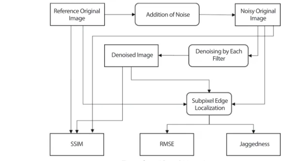
The overall flow of this study is shown in Fig. 1.

In the figure, the texts in rectangles indicate the input

or output data and the texts in rounded rectangles

the processes. As shown in Fig. 1, the evaluation of

denoising filters uses a reference original images as

ground truth data. Then, the reference original image is contaminated by addition of a certain type of noises.

In this study, Gaussian random noises were added to the reference original image for experiments. The resulting image becomes a noisy original image. The noisy original image is denoised by each tested filter.

The output of the denoising process is a denoised image. After the denoising process, the SSIMs of the noisy original image and the denoised images with their reference original image as ground truth data are calculated. SSIM is a widely used measure to evaluate the quality of image with reference to ground truth image.

Then, for evaluating the performance of denoising filters based on edge location, the following procedure is proposed. First, subpixel edge localization is performed for the edge locations in the reference original image, the noisy original image, and the denoised image by applying AWG proposed in Seo (2018), because it is considered the most accurate method among the subpixel edge localization methods and much faster than the Erf fitting method proposed in Hagara and Kulla (2011). Accordingly, the edge locations determined in the noisy original image and the denoised image are compared with the edge

locations determined in the reference original image.

The comparison is performed in two ways. First, the RMSE of the edge locations in the noisy original image and the denoised image is calculated with reference to the edge locations in the reference original image. The RMSE is calculated as:

RMSE = (1) where f

and g

are the reference and test edge locations, respectively, and N is the total number of edge locations.

Second, a measure proposed in this study is the jaggedness which measures the degree of fluctuation of the edge locations in the noisy original image and the denoised image with reference to the edge locations in the reference original image.

∑

(g

– f

)

N

Fig. 2. Jaggedness of edge locations.

Reference Original

Image Addition of Noise Noisy Original

Image

Denoised Image Denoising by Each

Filter

Subpixel Edge Localization

SSIM RMSE Jaggedness

Refere

nce e dge

Test e dge

x

x

x

The jaggedness is calculated as follows. As shown in Fig. 2, the signed distance of edge location in a test image at each edge location from the edge location in a reference image is calculated as x

, x

, and x

at edge locations, k–1, k, and, k+1, respectively. Then, the following two differences are calculated at edge location k as:

d

= x

– x

d

= x

– x

(2) Then, if both d

and d

are not zero and their multiplication d

· d

< 0, then the count of jaggedness increases by one. Thus, in the case shown in Fig. 2, the jaggedness count increases by one at edge location k.

This procedure is performed for all the given edge locations except the first and last edge locations. Then, the degree of jaggedness of edge locations in an image is calculated as:

Jaggedness (%)= × 100 (3)

where N is the total number of edge locations.

After obtaining SSIM, RMSE, and jaggedness of denoised image, denoising filters are evaluated based on those measures.

3. Experimental Results 1) Experiments with simulated images

In order to evaluate the denoising filters based on edge locations, a set of simulated edge images were generated for experiments. Experiments with simulated edge images are considered to be important because we know the ground truth edge locations in simulated edge images and thus we can measure absolutely the errors of edge locations in their denoised images.

For generating simulated edge images, a normal line equation for an edge is modeled as:

ρ = c

cosθ + r

sinθ (4)

where θ is the edge normal angle with reference to the column axis in the clockwise direction, (r

, c

) the coordinates of the center point of the simulated edge image, and ρ the distance from the origin to the edge which passes through the center point. Then, the following distance is calculated at all image pixel locations (r, c) as:

D(r, c) = (5) where σ

is the blurring factor, which was set to 1.0 in this study. Although an edge model with two blur parameters describes more completely the real imaged edge profiles (Seo, 2018a), one blur edge model is used in this study for simplicity.

Then, intensity at each pixel is calculated as:

I(r, c) = [erf(D(r, c)) + 1] (6) where erf(·) is the error function.

The simulated edge image generated by Eq. (6) is considered as the reference original image or ground truth edge image in this study. Then, a noisy original image is generated by adding Gaussian random noises to the reference original image as:

I

(r, c) = I(r, c) + n(r, c) (7) where the noise n(r, c) follows the Gaussian normal distribution as:

n(r, c) ~ N(0, σ

) (8) where σ

denotes the noise strength and was set to 0.01, 0.03, 0.05, 0.1, 0.15, and 0.2.

Fig. 3 show examples of generated noisy original edge images with contrast k=1.0 and noise strength σ

=0.1 with four different edge normal angles.

Then, each original noisy image was denoised by denoising filters: AF, BF, GF, WGF, WMP, and smoothing filter (SF). SF is a widely used filter to smooth images with the Gaussian blurring.

For implementation of the denoising filters, the parameters of each filter were tuned to remove similar No. of jagged location

N – 2

ccosθ + rsinθ – ρ 2 σ

K 2

amount of noises by visual inspection and the set of same values of the parameters was applied to all tested images for consistency of parameters. The role of each parameter in the denoising filters was described in Seo (2020b). In AF, κ indicates the factor to divide the intensity difference between central pixel and its neighborhood pixels in the exponential function (Perona and Malik, 1990). λ is the factor to control the conduction speed. In BF, S is the Gaussian blur factor in the spatial domain, and r is the Gaussian blur factor in the range domain. In GF, r denotes a blur factor in the spatial domain, and ε the square of the blur factor in the range domain. In WGF, r indicates a blur factor in the spatial domain, and λ the square of the blur factor in the range domain. In WMP, Ω denotes the size of the neighborhood used to calculate the weighted mean of patches. For AF, κ and λ were set to 0.4 and 0.1, respectively and the number of iterations was set to 10. For BF, S and r were set to 4 and 0.1, respectively. For GF, r and ε were set to 2 and 0.05, respectively. For WGF, r and λ were set to 2 and 0.05, respectively. For WMP, Ω was set to 5×5 pixels. The smoothing factor σ

in SF was set to 1.5.

Fig. 4 shows the images resulting from the application

of the denoising filters to a noisy original image.

As shown in Fig. 4, it is difficult to evaluate the quality of denoised images by human vision. This difficulty can be one of the reasons to use a computerized measure SSIM. Fig. 5 shows the SSIMs of the denoised images with reference to their reference original images. In Fig. 5, Original indicates the plots for the noisy original images. As shown in Fig. 5, the value of SSIM decreases rapidly as the noise strength increase from 0.01 to 0.2. The enhancement of SSIM values was

σn=0.1 and line normal angle θ=22°. (a) AF; (b) BF; (c) GF; (d) WGF; (e) WMP; (f) SF.

(a) (b) (c) (d) Fig. 3. Simulated edge images with contrast k=1.0 and noise strength σn=0.1.

(a) θ=0°; (b) θ=22°; (c) θ=46°; (d) θ=80°.

Fig. 5. SSIM of the denoised versions of the simulated edge images with reference to their ground truth images.

1 0.9 0.8 0.7 0.6 0.5 0.4 0.3 0.2 0.1 0

SSIM

0 0.05 0.1 0.15 0.2 Noise Strength

Original AF BF GF WGF WMP SF

distinct when denoising filters were applied. Among the denoising filters, AF and SF were shown to produce relatively higher SSIMs than other filters when the noise strength was relatively high. But this observation does not provide well the information about the geometric quality of the denoised images.

For evaluating the geometric quality of the denoised images, edge locations in the denoised

images were calculated by applying AWG to the denoised images. Fig. 6 shows one example of the edge locations determined by AWG in the denoised images, where location 0 is the ground truth location of the corresponding edge position. According to the plots in Fig. 6. SF was shown to produce the most accurate edge location among the denoising filters at the given position. In order to investigate the overall

Fig. 6. Example of edge profiles and their edge locations determined by AWG at an edge position in the denoised versions of a simulated edge image. The vertical lines indicate the edge locations determined by AWG for their corresponding edge profiles at the position.

1.2

1

0.8

0.6

0.4

0.2

0

-0.2

-6 -4 -2 0 2 4 6 X (pixels)

Intensity

Original AF BF GF WGF WMP SF

(a) (b)

Fig. 7. Edge location shift x determined by AWG for the denoised versions of noised edge images for the simulated edge image with contrast k=1.0, noise strength σn=0.1 and line normal angle θ=22°. (a) and (b) show the edge shift within two different ranges in the given edge.

0.8 0.6

0.4

0.2 0

-0.2

-0.4 -0.6

-0.8

0.8 0.6

0.4

0.2 0

-0.2

-0.4 -0.6

-0.8

x (pixels) x (pixels)

Original AF BF GF WGF WMP SF Reference

Original AF BF GF WGF WMP SF Reference 20 25 30 35 40

Distance along the Edge (pixels)

58 60 62 64 66 68 70 72 74 76 Distance along the Edge (pixels)

accuracy of edge locations in the denoised images, all edge locations were examined.

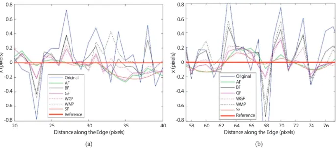
Fig. 7 shows examples of the edge location shifts within some given ranges along an edge feature in the denoised images. As shown in Fig. 7, AF and SF were shown to produce small edge location shifts as compared to other denoising filters in the given ranges.

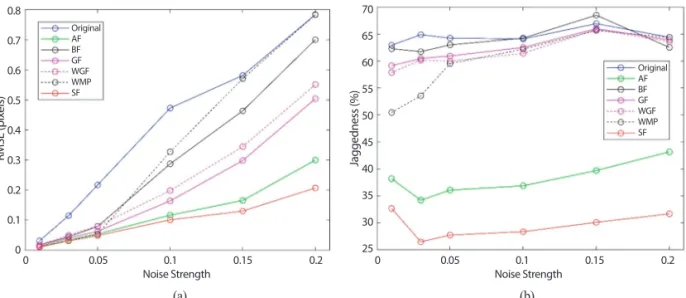
For further investigation of the quality of the edge locations in the denoised images, their RMSEs and jaggedness were calculated. Fig. 8 shows their RMSEs and jaggedness. The values of the RMSEs and jaggedness in Fig. 8 are the mean values of the RMSEs and jaggedness of the cases of the four different edge normal angles. According to the RMSE values in Fig. 8(a), SF can be considered as the most accurate method among the tested denoising filters in terms of edge location. Additionally, according to the jaggedness shown in Fig. 8(b), SF can also be

considered to produce edge locations with the highest geometric stability among the tested denoising filters in terms of edge locations.

2) Experiments with natural images

The denoising filters were also tested with natural images. The natural images were captured with a digital single-lens reflex camera. Then, the red band images in the images were used for experiments in this study.

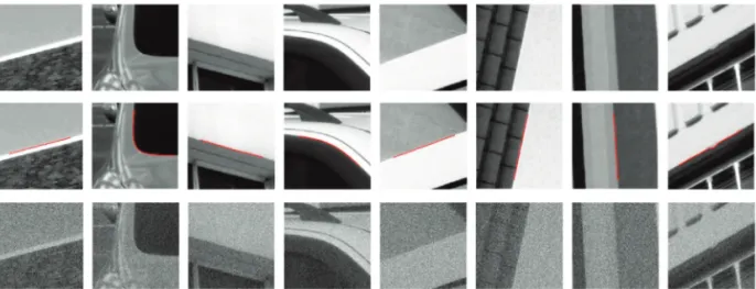
The test image was set to range [0,1] by dividing the images by 255. For the experiments, image chips in the test images were collected as shown in Fig. 9. As shown in Fig. 9, a total of 8 image chips were obtained from the four images and considered as the reference original images.

Fig. 10 shows the image chips, the image chips with reference locations of edges, and the images contaminated by noise σ

=0.1.

(a) (b)

Fig. 8. (a) RMSE of edge locations; (b) Jaggedness of edge locations after different denoising methods for the simulated edge images.

0.8

0.7

0.6

0.5

0.4

0.3

0.2

0.1

0

70 65 60 55 50 45 40 35 30 25

Jaggedness (%)

RMSE (pixels)

Original AF BF GF WGF WMP SF

Original AF BF GF WGF WMP SF

0 0.05 0.1 0.15 0.2 Noise Strength

0 0.05 0.1 0.15 0.2 Noise Strength

Fig. 9. Locations of the image chips in natural images.

Then, the noisy original image was denoised by the tested denoising filters: AF, BF, GF, WGF, WMP, and SF. The parameters of each filter were set to the same values used for denoising the simulated edge images.

Fig. 11 shows examples of the denoising results by applying all the tested filters to the natural image chip 2.

Fig. 12 shows SSIMs of the denoised images with reference to their reference original images. As shown in Fig. 12, AF and SF were shown to produce highest SSIMs across all the natural image chips. It is noteworthy that the SSIM of the noisy original images were very low with reference to the reference original image but the SSIMs of the images obtained by applying AF and SF to the noisy original images became very high. This indicates the importance of an efficient denoising filter for processing a noisy image.

However, it is difficult to determine the geometric

quality of edges in detail with the SSIM plots shown in Fig. 12.

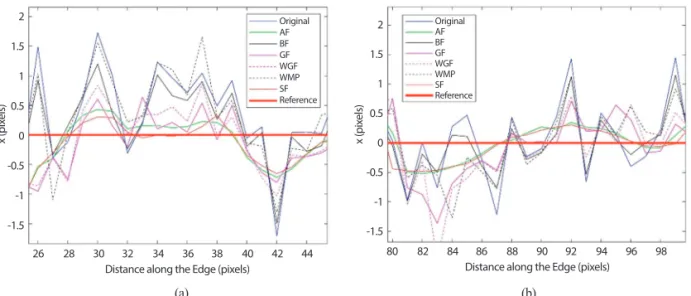
Fig. 13 shows the edge location shifts remaining in the denoised images with reference to the edge locations in the reference original images. The edge

chips contaminated by noise σn=0.1. From left to right: image chips 1 to 8, respectively.

(a) (b) (c) (d) (e) (f) Fig. 11. Images generated by different denoising methods for the natural image chip 2 contaminated by noise σn=0.1.

(a) AF; (b) BF; (c) GF; (d) WGF; (e) WMP; (f) SF.

Fig. 12. SSIM of the denoised versions of the noise- contaminated real images with reference to their ground truth images.

0.9 0.8 0.7 0.6 0.5 0.4 0.3 0.2 0.1

SSIM

1 2 3 4 5 6 7 8 Image Chip ID

Original AF BF GF WGF WMP SF

locations in the reference original image, the noisy original image, and the denoised images were determined by AWG. For applying AWG to the reference original images, the reference original images were smoothed by a Gaussian smoothing with blurring factor σ

=1.0. Subpixel edge localization for the noisy original images and the denoised images was applied directly to the images without smoothing in order to obtain the pure effect of each denoising filter on edge locations. As shown in Fig. 13, the edge location shifts

remaining in the denoised images with reference to the edge locations in their reference original images show that SF produced most accurate denoising results as compared to the other filters for the given edge ranges.

Fig. 14 shows the RMSEs and jaggedness of the edge locations in the denoised images. As shown in Fig. 14(a), AF and SF produced the most accurate edge locations after denoising. However, the advantage of SF against AF was not shown clearly in Fig. 14(a). The advantages of AF and SF were shown clearly in Fig.

(a) (b)

Fig. 13. Edge location shift x determined by AWG for the denoised versions of noised edge images for the natural image chip 2. (a) and (b) show the edge shift within two different ranges in the given edge.

2

1.5

1

0.5

0

-0.5

-1

-1.5

2

1.5 1

0.5

0 -0.5

-1

-1.5

x (pixels) x (pixels)

Original AF BF GF WGF WMP SF Reference

Original AF BF GF WGF WMP SF Reference

26 28 30 32 34 36 38 40 42 44 Distance along the Edge (pixels)

80 82 84 86 88 90 92 94 96 98 Distance along the Edge (pixels)

(a) (b)

Fig. 14. (a) RMSE of edge locations; (b) Jaggedness of edge locations after different denoising methods for the real image chips.

2.2 2 1.8 1.6 1.4 1.2 1 0.8 0.6 0.4 0.2

70 65 60 55 50 45 40 35 30 25 20

RMSE (pixels) Jaggedness (%)

Original AF BF GF WGF WMP

SF Original

AF BF GF WGF WMP SF

1 2 3 4 5 6 7 8 Image Chip ID

1 2 3 4 5 6 7 8 Image Chip ID

14(b), where the jaggedness of AF and SF was shown to be much lower than the other filters. Additionally, Fig. 14(b) shows that the jaggedness values of SF were lower than those of AF across all the natural image chips except image chip 7. This indicates the superiority of SF over AF in many cases in terms of geometric quality of edge locations.

4. Conclusions

In this paper, the quality of denoised images was evaluated by SSIM, RMSE, and jaggedness. RMSE and jaggedness were found to be useful to evaluate the quality of denoised images by providing ways to evaluate denoising filters in terms of their geometric accuracy. Among the tested denoising filters, AF and SF were found to recover edge locations better than the other tested filters in terms of RMSE. In addition, the proposed jaggedness measure was found to be useful to evaluate the distribution of tested edge locations with reference to ground truth edge locations. SF was found to produce slightly better edge locations than AF and much better than the other tested filters. Thus, SF can be considered as the most stable and accurate denoising method among the tested denoising filters in terms of geometric accuracy. This evaluation of jaggedness is related to the quality of feature extraction because the quality of edge location linking depends on the quality of distribution of edge locations. However, because the experiments were performed with the denoising filters tuned for a set of given conditions, the experiments can be considered to have some limitations on the comprehensive evaluation of the performance of denoising filters. Thus, further studies with setting their parameters to varying values under varying conditions will help a more complete evaluation of denoising filters.

Acknowledgements

This research was supported by Basic Science Research Program through the National Research Foundation of Korea (NRF) funded by the Ministry of Education (2016R1D1A1B02011625).

References

Aurich, V. and J. Weule, 1995. Non-linear gaussian filters performing edge preserving diffusion, In: Sagerer, G., Posch, S., Kummert, F. (eds), Mustererkennung 1995, Springer, Berlin, Heidelberg, Germany, pp. 538-545.

Canny, J., 1986. A computational approach to edge detection, IEEE Transactions on Pattern Analysis and Machine Intelligence, PAMI-8(6): 679-698.

Dong, L., J. Zhou, and G. Zhai, 2017. Efficient image sensor noise estimation via iterative re-weighted least squares, Proc. of IEEE Conference on Multimedia and Expo, Hong Kong, China, Jul.

10-14, pp. 1326-1331.

Hagara, M. and P. Kulla, 2011. Edge detection with sub-pixel accuracy based on approximation of edge with Erf function, Radioengineering, 20(2): 516-524.

He, K., J. Sun, and X. Tang, 2013. Guided image filtering, IEEE Transactions on Pattern Analysis and Machine Intelligence, 35(6): 1397-1409.

Li, Z., J. Zheng, Z. Zhu, W. Yao, and S. Wu, 2015. Weighted guided image filtering, IEEE Transactions on Image Processing, 24(1):

120-129.

Perona, P. and J. Malik, 1990. Scale-space and edge detection using anisotropic diffusion, IEEE Transactions on Pattern Analysis and Machine Intelligence, 12(7): 629-639.

Porikli, F., 2008. Constant time O(1) bilateral filtering,

Proc. of IEEE Conference on Computer Vision

and Pattern Recognition, Anchorage, AK, Jun.

23-28, pp. 1-8.

Rashe, C., 2018. Rapid contour detection for image classification, IET Image Processing, 12(4):

532-538.

Sapiro, G. and D.L. Ringach, 1996. Anisotropic diffusion of multivalued images with applications to color images, IEEE Transactions on Image Processing, 5(11): 1582-1586.

Seo, S., 2017a. Prediction of edge displacement due to image contrast, Photogrammetric Record, 32(158): 119-140.

Seo, S., 2017b. Estimation of edge displacement against brightness and camera-to-object distance, IET Image Processing, 11(8): 568-577.

Seo, S., 2018a. Edge modeling by two blur parameters in varying contrasts, IEEE Transactions on Image Processing, 27(6): 2701-2714.

Seo, S., 2018b. Subpixel edge localization based on adaptive weighting of gradients, IEEE Transactions on Image Processing, 27(11):

5501-5513.

Seo, S., 2019. Subpixel line localization with normalized sums of gradients and location linking with straightness and omni-directionality, IEEE

Access, 7: 180155-180167.

Seo, S., 2020a. Line-detection based on the sum of gradient angle differences, Applied Sciences, 10(1): 254.

Seo, S., 2020b. Image denoising and refinement based on an iteratively reweighted least squares filter, KSCE Journal of Civil Engineering, 24(3):

943-953.

Smith, S. and J.M. Brady, 1997. SUSAN: A new approach to low level image processing, International Journal of Computer Vision, 23(1): 45-78.

Steger, C., 1998. An unbiased detector of curvilinear structures, IEEE Transactions on Pattern Analysis and Machine Intelligence, 20(2): 113-125.

Tomasi, C. and R. Manduchi, 1998. Bilateral filtering for gray and color images, Proc. of International Conference on Computer Vision, Bombay, India, Jan. 7, pp. 839-846.

Wang, Z., A.C. Bovik, H.R. Sheikh, and E.P.

Simoncelli, 2004. Image quality assessment:

From error visibility to structural similarity, IEEE Transactions on Image Processing, 13(4):

600-612.