파이프라인을 이용한 이산화탄소 수송에서 중간 저장 허브 선정 모델링 및 시각화를 위한 시뮬레이터 개발
Development of a Simulator for the Intermediate Storage Hub Selection Modeling and Visualization of Carbon Dioxide Transport Using a Pipeline
이지용
한국과학기술원 산업 및 시스템 공학과 Ji-Yong Lee([email protected]) 요약
이산화탄소 포집 및 저장 / 격리 (CCS) 기술은 많은 이산화탄소 저감 방법 중 이상적인 방법으로 주목 받고 있다. 이산화탄소를 포집해서 파이프라인을 통해 저장소까지 수송할 때, 저장소가 가까운 경우 직접 수송할 수도 있지만, 중간 저장의 역할을 하는 허브를 거쳐 수송할 수도 있다. 허브의 수와 위치를 결정하는 것은 중요한 문제이다. 다목적 의사 결정을 위한 수학 모델은 많은 제약식과 목적식을 수반하는데, 문제의 계산 복잡도가 증가하지만 항상 최적을 보장하지 않는다. 본 연구에서는, 이산화탄소 수송망에서 중간 저장
허브의 위치와 수를 결정하는 알고리즘을 제안하고, 이를 활용하여 이산화탄소 발생지의 연결 네트워크 시
뮬레이터를 개발한다. 시뮬레이터에서는 또한 이산화탄소의 수송 경로를 제공한다. 사례 연구로 한국에 모 델을 적용한다.
■ 중심어 :∣이산화탄소 포집 및 저장 / 격리 (CCS)∣수송망∣중간 저장 허브∣파이프라인 수송∣시뮬레이터∣
Abstract
Carbon dioxide Capture and Storage/Sequestration (CCS) technology has attracted attention as an ideal method for most carbon dioxide reduction needs. When the collected carbon dioxide is transported to storage via pipelines, the direct transport is made if the storage is close, otherwise it can also be transported via an intermediate storage hub. Determining the number and the location of the intermediate storage hubs is an important problem. A decision-making algorithm using a mathematical model for solving the problem requires considerably more variables and constraints to describe the multi-objective decision, but the computational complexity of the problem increases and it also does not guarantee the optimality. This research proposes an algorithm to determine the location and the number of the intermediate storage hub and develop a simulator for the connection network of the carbon dioxide emission site. The simulator also provides the course of transportation of the carbon dioxide. As a case study, this model is applied to Korea.
■ keyword :∣Carbon Dioxide Capture and Storage/Sequestration (CCS)∣Transport Network∣Intermediate Storage Hub∣Pipeline Transportation∣Simulator∣
접수일자 : 2016년 05월 16일 수정일자 : 2016년 10월 05일
심사완료일 : 2016년 10월 05일
교신저자 : 이지용, e-mail : [email protected]
I. Introduction
As global warming has worsened, the whole world has been forced to reduce CO2 emissions, which are the major cause of global warming. According to reports released by the Intergovernmental Panel on Climate Change (IPCC), Carbon dioxide Capture and Storage/Sequestration (CCS) is expected to be the most contributive technology among the CO2 reduction methods[1]. CCS is predicted to be able to reduce the CO2 emission rate by at least 15% and at most 55%
by 2100[2]. CO2 capture technology, which accounts for 70–80% of the CCS cost, is a core technology with examples such as pre-combustion and post-combustion capture technology and oxy-fuel combustion technology [3][4]. Sequestration technologies, as a technique for storing CO2 in deep seabeds or land, have been actively researched to solve the problems inherent in the storage system's compatibility and stability[5].
In contrast, relatively little research on pipeline transportation technology for CO2 has been conducted.
As pipelines are sometimes installed in densely populated and residential areas, and through rivers and mountainous terrain, it is necessary to analyze not only the routes’
cost effectiveness, but also the pipeline equipment.
Although the ratio of the cost as a percentage of the entire CCS system might be small, the accurate analysis of a pipeline transportation network can result in a large cost savings compared with other techniques, ensuring the stability of a long-term CCS project[6].
The existing interstate natural gas pipelines in U.S.
operate in the Central Region (Iota, Utah, Wyoming and etc) with interconnections to the interstate network that also serve a large domestic natural gas.
These have developed around several local hubs, the largest being the Carthage, Henry, and Egan hubs located in eastern Texas and southwestern Louisiana[7][8].
The role of these hubs is to provide support to local region needing natural gas transportation service more efficiently.
In the CCS system like the preceding natural gas case, locating intermediate hub is necessary. and one source can be connected to the only one hub.
Many researchers have proposed a cost model for the pipeline technology that is a function of the diameter of the pipeline, CO2 flow rate, and the pipeline length, assuming a one-to-one transport from CO2 emission sources to the sequestration plant[9-11].
To make a pipeline an efficient means of transport, it is suggested that hub storages play a role as an interim storage between CO2 emission sources. Each hub node can re-transport the collected CO2 to the sequestration sites. Intermediate storage hubs are needed to safely and efficiently transport CO2 via pipelines and to connect each site cost effectively.
The characteristics of the pipelines affected by CO2 properties strongly influence the location and the number of intermediate hubs, which is one of the most important issues across the whole CCS system[12][26].
And typically many studies of facility location problem have done providing mathematical formulations or heuristic algorithms[13-15]. Generally, a decision- making algorithm using a mathematical model for solving the problem requires considerably more variables and constraints to describe the multi-objective decision, but the computational complexity of the problem increases and then it also does not guarantee the optimality to determine the number and the location of the intermediate storage hubs. So, approximation algorithm such as greedy heuristics and local search technique were proposed for facility location problems[13-18].
The case that it costs high to connect each node and locate hubs does not always guarantee the optimal policies because of mathematically undefined factors and current national policies. Therefore, this
research proposes a simple local search algorithm to easily determine the location and the number of the intermediate storage hub and an important contribution is to develop a simulator for the connection network of the source to the sink. It is given as an example of the course of transportation of the carbon dioxide.
II. Problem definition
1. Description of the CO2 emission source node
Industries capturing CO2 are classified as power plants, iron steel plants, oil refinery plants, and petrochemical plants.
[Table 1] represents the unit cost to collect 1 ton of CO2, the capture capital costs, and maximum capacity. The location problem of the intermediate hubs regards these factors for the cost-effective connection among them and re-distribute CO2.
Power plants [19]
Iron and steel plants [20]
Oil refinery plants [21]
Petrochemical plants
[22]
Capacity
(tCO2/y) 1,480,000 2,795,000 1,013,000 969,000 Capture
capital cost (million $)
333 639 283 558
Unit capture cost
($/t CO2)
49.76 38.29 80.26 58.85
Table 1. Capital and unit capture costs of CO2
capture technology according to each industry
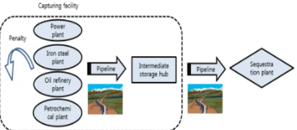
The distribution of the captured CO2 generates decision problems, such as how many hubs are needed, where the hubs are located, and how to connect the capture plants and the hubs. To determine the number and the hub location in the CCS system, [Figure 1] illustrates the schematic description of the hub selection, which is only affected
by the network connection between the CO2 emission sources and hubs.
Fig. 1. Schematic description of the hub selection
When CO2 flows via pipelines, the various terrain conditions are considered. For example, installing a pipeline to the plains, it is different from doing so in areas with dense populations, mountains, or rivers, etc. By considering the cost factor of meeting the topographical conditions associated with the aforementioned differences in terrain, it is assumed that the network design can vary with the topographical conditions. [Table 2] presents a rough estimate for the costs of pipelines in various terrains, based on the topographical requirements to lay pipelines between the capturing sites and hubs.
Terrain Cost multiplier
Flat open countryside 1.0
Mountainous 2.5
Desert 1.3
Forest 3.0
Offshore (up to 500 m water depth) 1.6 Offshore (above 500 m water depth) 2.7 Table 2. Costs of pipelines in various terrains[23]
2. Description of the hub node
The candidate hub nodes are the locations selected in advance by the researchers based on the conditions of the study, geography, CO2 emission node distribution, and etc. In the case of CO2 transportation problem, the arcs connecting up with source nodes and hub nodes are pipelines for which capital cost is
expensive, so basic assumption for the model is that single source can be connected to single hub.
A hub node is selected from among the candidate hub nodes, the constraints for which are the storable capacity and maximum length of the pipeline that can cover the CO2 emission source node around each candidate hub node.
The maximum radius centered by the hub nodes is limited when it forms a cluster in the center hub.
Equation (1) expresses the distance constraints of the capable pipeline connection lengths from the candidate hubs to the CO2 emission sites, which are less than the maximum ranges of the candidate hubs:
≤ ∀∀ (1)
where is the distance from CO2 emission source i to candidate hub j and is the maximum capable pipeline length from candidate hub j.
Equation (2) states the capacity restriction at each candidate hub site, where is the amount of emitted CO2 to be transported from CO2 emission source i to candidate hub site j and is the maximum level of storage achieved by candidate hub j.
≤ ∀ (2)
When the CO2 emission source node is connected to the candidate hub node, it is important to satisfy the storage capacity of the candidate hub as expressed in Equation (2). To form a cluster in which the centripetal points have a radius around a candidate hub node, the pipeline is connected to the CO2 emission source node of the cluster within.
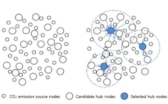
[Figure 2] provides a simple description of the distributed CO2 emission source nodes and candidate hub nodes.
Fig. 2. Description of CO2 emission source and candidate hub nodes
Ⅲ. Hub selection model
In this section, a hub selection model is proposed to determine the realized hub node from the candidate hub nodes. It must be possible to process all of the CO2 emission source nodes using the CCS system, as far as possible.
The purpose for the development of the model is to minimize total cost during the CCS system’s processing period. Because they are critical to the decisions regarding the number of hub nodes and the hub locations, the candidate hubs must be based on a more realistic assumption. The more CO2 emission source nodes there are in the cluster centered by a candidate hub node, the more importance granted to the positions of the candidate hub nodes and the total amount of CO2.
However, under the aforementioned CO2 emission conditions, it cannot be explained how CO2 emission source nodes are successively connected. If CO2 emission source nodes are randomly dispersed, each node has a priority of connection to the hub nodes.
The particular algorithm and formula are proposed to handle it by Pagerank theory[24].
With the assumptions described above, a form of the rank equation for the candidate hub nodes is as follows:
∀ (3) where n is the number of hub nodes defined and
is the number of CO2 emission source nodes in the cluster from candidate hub j in step n. is the transpose matrix of in which the entry in the row and column is
∈
∀∀
(4)
is the number of out-links from CO2 emission source node i to candidate hub node j. Likewise,
is the matrix in which the entry in the row and column is
∈
∀∀
(5)
where and are the amount of emitted CO2 to be transported and the distance from CO2 emission source i to candidate hub node j. To explaining this algorithm, [Table 3] provides the node descriptions of the example for calculating the value of .
CO2
amount (tCO2)
Distance (km) Candidate
hub 1
Candidate hub 2
Candidate hub 3
CO2 emission node1 100 20 - -
CO2 emission node2 180 30 15 -
CO2 emission node3 300 50 10 25
CO2 emission node4 90 15 - 30
CO2 emission node5 160 - 20 40
CO2 emission node6 200 - 40 -
Table 3. Source node descriptions in the example
The purpose of this example is to line up the rank
value and select two hub nodes from among three candidate hub nodes. There are six CO2 emission source nodes which emit a total of 1030t CO2 and three candidate hub nodes. Based on the
above data, the possible connection of each node is as shown in [Figure 3].
Fig. 3. Simple example of a hub selection problem - Step 1
In [Figure 3], the candidate hub nodes and the CO2 emission source nodes are presented as blue circles and white circles. The red arrows represent the possibility of laying the pipeline between the nodes in a circle. The dashed blue lines reflect the boundaries of the imaginary clusters which are given by researchers.
The existing CO2 emission source nodes within candidate hub 1 are nodes 1, 2, 3, and 4. Likewise,
can be defined as follows:
(6)
CO2 emission source node1 is only connected to H1, whereas node 2 has possible connections with H1 and H2. The connectivity matrix and the resulting matrix of are
(7)
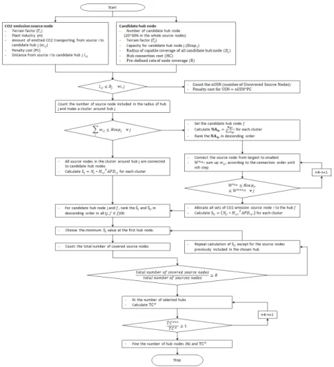
Fig. 5. Flow chart of the hub selection model The result of Step 1 is obtained according to the
following values:
(8) Equation (8) shows H2 has the largest value and is therefore selected for the first tume from among all of the candidate hub nodes. The next step is to choose another hub node except H2.
The algorithm repeats the operations described above with the remaining candidate hub nodes to connect the rest of the CO2 source nodes and candidate hubs. The result can be seen in [Figure 4].
Fig. 4. Simple example of a hub selection problem - Step 2
The following equations are the same as above.
(9)
(10)
The result of Step 2 is obtained by .
(11)
The second hub node is H1.
[Figure 5] describes a flow chart of clustering algorithm with candidate hub nodes as the center aggregating all of the assumptions aforementioned.
IV. Simulation results
1. Data set
[Table 4] gives the information of the intermediate storage hubs like storage capital cost and CO2 unit storage costs.
Storage facility (steel tank) Storage capital cost($) 10,228,607 Unit storage cost ($/t CO2) 0.72
Table 4. Capital and unit storage costs of CO2
storage facilities [11]
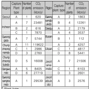
The data set for the CO2 emission sites of Korea case is as shown in [Table 5] presents how many plants are located in each district considering capture plant types and the amount of CO2 emitted.
Region Capture
Plant type
Number of plants
CO2
emission (kton/y)
Region Capture plant type
Number of plants
CO2
emission (kton/y)
Seoul A 1 620 Gyeong
sangb ukdo
A 2 1863
Incheon
A 7 23481 B 4 12261
B 2 616 Daegu A 2 2179
C 1 7870
Busan
A 4 3537
Gyeong
gido A 7 5744 B 1 112
Chung cheong namdo
A 11 119622
Ulsan
A 2 4257
C 1 2986 C 1 4817
D 3 2760 D 8 5441
Chung cheong
bukdo
D 5 16008 Jeoll ana mdo
A 7 21506
Gangwo ndo
A 5 8405 C 1 6103
D 6 27719 D 3 2601
Gyeong sangna
mdo
A 1 29539
Jeoll abuk do
A 3 2576
* Plant type
A: Power plant facility / B: Iron and steel plant facility C: Oil refinery plant facility/ D: Petrochemical plant facility Table 5. The number of capture facilities in each
administrative district and the amount of CO2 emissions [25]
Terrain conditions identified by the U.S. National Energy Technology Laboratory (NETL) are referred to the areas in which the CO2 emission sources are located and classified into the mountainous, flat, river, and high population for the Korean case. The conditions, in turn, affect the pipeline design and cost multipliers.
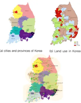
In this case study, Korea is divided into 13 cities and provinces according to the administrative district to define the industry groups and the amounts of CO2 they emit ([Figure 6](a)). Each district can be defined by one of the terrain conditions (mountainous, flat, river, and high population).
Researchers can select the locations of the candidate hub nodes by considering the distribution of nodes and amount of emitted CO2, or other policies. The number of candidate hub nodes is assumed to be 25% (22 nodes) of the total number of CO2 emission source nodes (88 nodes).
All the nodes are distributed in each district, as shown in [Figure 6](c). Green circles and yellow circles indicate CO2 emission source nodes and candidate hub nodes.
(a) cities and provinces of Korea (b) Land use in Korea
(c) Distribution of CO2 emission sources
Fig. 6. Description for the simulator in Korea case
2. Hub selection
One of the most important objective of this study is to use hub nodes to maximize coverage rates, which mean how many source nodes are connected to the hubs, and so the simulator calculates the number of nodes every time by the increase of the number of hubs. The minimum coverage rate is assumed more than 75% in the light of researchers' policies.
[Figure 7] provides the three coverage graphs derived from the algorithm. [Figure 7](a) shows the rate of the connected number of CO2 emission source nodes to the hub nodes depending on the number of hubs. When the number of hubs is set to more than 7, the coverage rate exceeds about 75% of the total and afterwards it increases slightly and stops in 8.
Thus, the minimum number of hub nodes can be set to 7. Likewise, the amount of emitted CO2 covered by the hub nodes is shown in [Figure 7](b) and [Figure 7](c) reveals how the total cost changes as the increase of the number of hubs.
(a) Coverage rate depending on the number of hubs
(b) Percentage of covered amount of CO2
(c) Cost for pipeline transportation depending on the number of hubs
Fig. 7. Coverage rates of CO2 emission source nodes depending on the number of hubs
[Figure 8] provides linkage maps of all of the nodes connecting via a cost analysis and coverage rate by selecting hubs with the assumptions. If the assumptions like the hub cluster radius, distribution of nodes, terrain factors, and other cost factors are changed, this simulator can give intuitive result for a decision making.
Fig. 8. Linkage map of pipeline connection network
V. Conclusion and directions for furture research
CCS is a technology for capturing, transporting,
and storing/sequestrating emitted CO2 from fuel combustion at some isolated site. Previous studies have focused on infrastructural technologies involving pipeline design parameters, which can influence the cost of designing cost estimation models for the CO2 pipelines based on the various problems’ definitions and assumptions.
The primary purpose is to minimize total cost of CCS systems. Actually, one of considerable thing is to satisfy minimum coverage rate of overall source nodes which means that pre-determined minimum coverage rate should be satisfied within a system.
The minimum coverage rate is determined by researchers or a national policy to set the attainment of the goal in that globally mitigating greenhouse effect.
The purpose of this study is to provide an algorithm for placing the intermediate hub storage and develop a simulator to visualize how they are connected. The algorithm and developed simulator have simple assumption and give intuitive decision making process with obtaining the number and positions of hubs.
CCS is expected to be the most contributive technology among the CO2 reduction methods. From a business perspective, it can also be applied to the other cases such as US, China or other districts. It is obvious that future research opportunities which consider undetermined cost factors and improve the algorithm are relevant for adaptable real cases for future research. Further, it might also be worthwhile to investigate settings where other industries can be of general application by extension.
참 고 문 헌
[1] IPCC, Climate Change 2014: Mitigation of Climate Change, Working Group Ⅲ Contribution
to the IPCC 5th Assessment Report, IPCC, Geneva, 2014
[2] IEA, World Energy Outlook 2009, OECD/IEA, Paris, 2009
[3] E. S. Rubin, IPCC special report on carbon dioxide capture and storage, RITE international workshop on CO2 geological storage, 2006.
[4] IEA Greenhouse Gas R&D Programme, Transmission of CO2 and Energy, Report no.PH4/6, 2002.
[5] E. S. Rubin, “Understanding the pitfalls of CCS cost estimates,” International Journal of Greenhouse Gas Control, Vol.10, pp.181-190, 2012.
[6] C. B. Farris, “Unusual design factors for supercritical CO2 pipelines,” Energy Progress Vol.3, pp.150-158, 1983.
[7] EIA, Annual Energy Outlook 2007, DOE/EIA-0383, February 2007.
[8] EIA, Natural Gas Market Centers and Hubs, DOE/EIA-0383, October 2003
[9] D. L. McCollum and J. M. Ogden, Techno- Economic Models for Carbon Dioxide Compression, Transport, and Storage and Correlations for Estimating Carbon Dioxide Density and Viscosity, Institute of Transportation Studies, University of California, Davis, 2006.
[10] M. M .J. Knoope, W. Guijt, A. Ramirez, and A.
P. C. Faaij, “Improved cost models for optimizing CO2 pipeline configuration for point-to-point pipelines and simple networks,”
International Journal of Greenhouse Gas Control, Vol.22, pp.25-46, 2014.
[11] Rickard Svensson, Mikael Odenberger, Filip Johnsson, Lars Strömberg, “Transportation systems for CO2 application to carbon capture and storage,” Energy Convention and Management, Vol.45, No.15-16, pp.2343-2353, 2004 [12] J. R. MacFarland and H. J. Herzog, “Incorporating carbon capture and storage technologies in
integrated assessment models,” Energy Economics, Vol.28, pp.632-652, 2006.
[13] G. Cornuejols, G. Nemhauser, and L. Wolsey, The uncapacitated facility location problem. InP.
Mirchandani and R. Francis, editors, Discrete Location Theory. John Wiley and Sons, 1990 [14] R. Love, J. Morris, and G. Wesolowsky,
Facilities Location: Models and Methods, North-Holland, New York, NY, 1988
[15] P. Mirchandani and R. Francis, editors. Discrete Location Theory, John Wiley and Sons, New York, NY, 1990.
[16] D. S. Hochbaum, "Heuristics for the xed cost median problem," Mathematica Programming, Vol.22, pp.148-162, 1982.
[17] K. Jain, M. Mahdian, E. Markakis, A. Saberi, and V. Vazirani, "Greedy facility location algorithms analyzed using dual tting factor revealing lp,"
To appear in the Journal of ACM.
[18] M. Korupolu, C. Plaxton, and R. Rajaraman, Analysis of a local search heuristic for facility location problems, Technical Report 98.30, DIMACS, 1998.
[19] E. S. Rubin and C. Chen, et al,. “Cost and performance of fossil fuel power plants with CO2 capture and storage,” Energy Policy, Vol.35, No.9, pp.4444-4454, 2007.
[20] J. A. V. Lie, T. Hcogg, M. B. Grainger, D. Kim, and T. Mejdell, “Optimization of a membrane process for CO2 capture in the steel making industry,” International Journal of Greenhouse Gas Control, Vol.1, No.3, pp.309-317, 2007.
[21] M. Gadalla and Z. Olujic, M. Jobson, R. Smith,
“Estimation and reduction of CO2 emission from crude oil distillation units,” Energy, Vol.31, pp.2062-2072, 2006.
[22] K. Mollersten and J. Yan, Jose R. Moreira,
“Potential market niches for biomass energy
with CO2 capture and storage–Opportunities for energy supply with negative CO2 emissions,” Biomass and Bioenergy, Vol.25, No.3, pp.273-285, 2003.
[23] IEA, World Energy Outlook 2010, OECD/IEA, Cancun, 7 Dec. 2010.
[24] Lawrence Page, Sergey Brin, Rajeev Motwani and Terry Winograd, “The PageRank Citation Ranking: Bringing Order to the Web,” 1998.
[25] IEA GHG CO2 database, 2006, http://www.iea.o rg/statistics/topics/co2emissions/
[26] J. H. Han and I. B. Lee, “Development of a scalable infrastructure model for planning electricity generation and CO2 mitigation strategies under mandated reduction of GHG emission,” Applied Energy, Vol.88, pp.5056-5068, 2011.
저 자 소 개
이 지 용(Ji-Yong Lee) 정회원
▪2007년 : 한국과학기술원(KAIST) 산업 및 시스템 공학과 졸업
▪2007년 ∼ 현재 : 한국과학기술 원(KAIST) 산업 및 시스템 공 학과 박사
<관심분야> : 생산관리, 경영정보시스템