Spatial Distribution Pattern of the Populations of Carex siderosticta at Mt.
Geumjeong and Mt. Ahop
Man Kyu Huh*
Department of Molecular Biology, College of Natural Sciences, Dong-eui University Box 995 Eomgwangno, Busan 614-714, Korea Received November 7, 2014 /Revised March 3, 2015 /Accepted March 4, 2015
Data on the spatial distribution of a plant population among administrative areas is useful for various purposes. In this study, I analyzed the spatial distribution of the geographical distances of Carex side- rosticta at Mt. Geumjeong and Mt. Ahop in Korea. The aim was to test a spatial structure within two populations of C. siderosticta. Most natural plots of C. siderosticta are not uniformly distributed in the forest community; for example, uniform plots were aggregately distributed within a space of 6.0 m
× 6.0 m. When the sampling plots were larger than 6.0 m × 12.0 m, the individuals of C. siderosticta were aggregately distributed. The neighboring patches of C. siderosticta were predominantly 7.5 m to 9.0 m apart, on average; however, if the natural populations were disturbed by human activities, the aggregation occurred in shorter distances than a scale of 9.0 m. Moran's I of C. siderosticta significantly differed from the expected value in only 16 of 40 cases (40%). In conclusion, the geographical dis- tribution of C. siderosticta is not even, with varying degrees of size in the plots, while human activities give rise to density effects in the plots at both Mt. Geumjeong and Mt. Ahop in Korea.
Key words : Carex siderosticta, Moran's I, neighboring patches, patchiness index, spatial autocorrelation
*Corresponding author
*Tel : +82-51-890-1529, Fax : +82-505-182-6870
*E-mail : [email protected]
This is an Open-Access article distributed under the terms of the Creative Commons Attribution Non-Commercial License (http://creativecommons.org/licenses/by-nc/3.0) which permits unrestricted non-commercial use, distribution, and reproduction in any medium, provided the original work is properly cited.
Journal of Life Science 2015 Vol. 25. No. 4. 369~375 DOI : http://dx.doi.org/10.5352/JLS.2015.25.4.369
Introduction
Knowledge of specific habitats is also critical in the study of the distribution of plants. Habitats include a combination of physical factors that represent the environmental con- ditions in which organisms live [10]. Each plant community was considered as a discrete patch occupied by individuals of different species from a limited regional pool because all species were assumed to be in competition with each other.
The spatial prediction of species distributions from survey data has recently been recognized as a significant component of conservation planning [8, 18].
Quantitative examination of spatially explicit data in ecol- ogy is broadly categorized as ‘‘spatial analysis’’ [13, 15]. The analysis of the spatial pattern of individuals of a particular species has long been a concern of ecologists [21].
Many ecologists have adopted several different major schools of spatial analysis from other disciplines [15]. The first of these comes from geography, and its methods include
the use of statistics (e.g., Moran’s I) to measure spatial auto- correlation [6, 19, 20]. It measures the degree to which the occurrence of an event in a real unit constrains, or makes more probable, the occurrence of an event in a neighboring areal unit.
Over the last decade, statistical ecologists have developed a number of elegant tools to incorporate spatial (or temporal) variables in analyses of multivariate ecological data sets. The presence of spatial (or temporal) autocorrelation in commun- ity composition data can be tested using multivariate Mantel correlograms. Variation partitioning [3, 17] provides a meth- od for distinguishing the separate (and combined) influences of environmental, spatial, and temporal variables on the var- iability of multi-species distribution and abundance data.
Carex siderosticta Hance is an herbaceous and belongs to the family, Cyperaceae. The fruits are achene and yel- low-flower blooms July–August in forests. Flowering culms and vegetative culms spaced; flowering culms clothed by bladeless sheaths at base, pale brown, without leaves. Leaf blades of vegetative culms are oblong-lanceolate, sometimes with white stripes. Flowering culms grow up to 30 cm tall.
C. siderosticta is a species of sedge native to East Asia [23].
In this report, the several statistical tools of percentage distribution and population structure of the geographical areas are used to study the spatial distribution of C. side- rosticta in Busan.
Mt. Geumjeong and Mt. Ahop locate in south of the Korean. A sample of a large (more than 500 individuals) natural population of C. siderosticta collected at both moun- tains and was used in this study. It is expected to provide useful experimental conditions because of the large undis- turbed and isolated site. Most temperate Carex species in- cluding C. siderosticta have shoots formed during the pre- vious year, some emerging in autumn, others remaining be- low ground until spring [2]. The maximum shoot life span for temperate species appears to be approximately 24 months but mortality is very high; sometimes 90% of shoots do not live for the whole 2-year life span. Mortality is caused by differences in time of emergence, flowering, animal graz- ing, the age of the genet, and internal competition through the rhizome system. Thus, C. siderosticta is ideal species to study the spatial distribution pattern of the population levels.
The purpose of this paper was to describe a statistical analysis for detecting a species association, which is valid even when the assumption of within- species spatial ran- domness is violated. The purpose of this study is addressed:
is there a spatial structure within two populations of C. side- rosticta? and 2) if so, what is the spatial pattern and is it the same for all populations?
Materials and Methods
Study areaI conducted the spatial analysis in the communities of Carex siderosticta at Mt. Geumjeong in Busan-si. The moun- tain (801.5 m) is highest in Busan. Mt. Ahop (350.0 m) locates in Gijang-gun, Busan-si, Korea. Mt. Geumjeong and Mt.
Ahop is about 20 km away. It has a temperate climate with a little hot and long summer. In this region the mean annual temperature is 14.7℃ with the maximum temperature being 29.4℃ in August and the minimum -0.6℃ in January. Mean annual precipitation is about 1519.1 mm with most rain fall- ing period between June and August.
Sampling procedure
Spatial ecologists use artificial sampling units (so-called quadrats) to determine abundance or density of species. The number of events per unit area are counted and divided by area of each square to get a measure of the intensity of each quadrat. I established many 1.5 m × 1.5 m quadrats with an area of 12 m × 12 m each around one area at Mt. Ahop
and Mt. Geumjeong. I randomly located quadrates in each plot which I established populations. The quadrat sizes were 1.5 m × 1.5 m, 1.5 m × 3 m, 3 m × 3 m, 3 m × 6 m, 6 m
× 6 m, 6 m × 12 m, and 12 m × 12 m. I mapped all plants to estimate C. siderosticta density per plot.
Index calculation and data analysis
The spatial pattern of C. siderosticta was analyzed accord- ing to the Neatest Neighbor Rule [5, 15] with Microsoft Excel 2010.
Average viewing distance (rA) was calculated as follows:
Where ri is the distance from the individual to its nearest neighbor. N is the total number of individuals within the quadrat.
The expectation value of mean distance of individuals within a quadrat (rB) was calculated as follows:
Where D is population density and D is the number of individuals per plot size.
R =
When R > 1, it is a uniform distribution, R = 1, it is a random distribution, R < 1, it is an aggregated distribution.
The significance index of the deviation of R that departs from the number of “1” is calculated from the following for- mula [14].
When CR > 1.96, the level of the significance index of the deviation of R is 5%, and When CR > 2.58, the level is 1%.
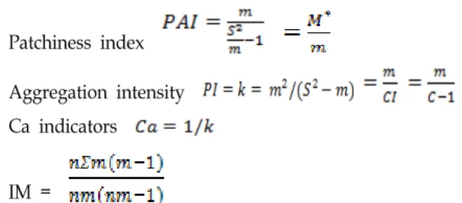
I calculated the degree of population aggregation under different sizes of plots by dispersion indices: index of clump- ing or the index of dispersion (C), aggregation index (CI), mean crowding (M*), patchiness index (PAI), negative bino- minal distribution index K, Ca indicators (Ca is the name of one index) [16] and Morisita index (IM) were calculated with Microsoft Excel 2010. The formulae are as follows:
Index of dispersion:
Aggregation index
Mean crowding = m + CI = m + C-1 -1
Table 1. Spatial patterns of Carex siderosticta individuals at different sampling quadrat sizes in Mt. Geumjeong and Mt. Ahop
Location Quadrat size (m × m) Density R CR Distribution pattern
Mt. Geumjeong 1.5×1.5
1.5×3 3×3 3×6 6×6 6×12
12×12 12×24
5.778 4.774 5.490 3.778 2.463 1.112 0.809 0.658
1.992 1.528 1.761 1.788 1.448 0.670 0.828 0.542
12.451 4.868 9.217 12.427 8.592 -7.496 -4.743 -11.514
Uniform Uniform Uniform Uniform Uniform Aggregation Aggregation Aggregation
Mt. Ahop 1.5×1.5
1.5×3 3×3 3×6 6×6 6×12
12×12 12×24
4.739 4.200 2.625 2.385 1.000 0.948 0.998 0.547
2.277 2.968 1.881 2.362 0.874 0.907 0.502 0.710
9.469 22.956 10.824 23.063 -0.874 -1.685 -0.603 -6.731
Uniform Uniform Uniform Uniform Aggregation Aggregation Aggregation Aggregation
Patchiness index
Aggregation intensity Ca indicators
IM =
Where S2 is variance and m is mean density of C.
siderosticta.
When , it means aggregately dis-
tributed, when , it means uniformly dis- tributed, when , it means aggregately dis- tributed, and when it means uniformly distributed.
The mean aggregation number to find the reason for the aggregation of C. siderosticta was calculated [1].
Where r is the value of chi-square when 2k is the degree of freedom and k is the aggregation intensity.
Spatial structure
Numerical simulations of previous analyses were per- formed to investigate the significant differences at various distance scales, i.e., 1.0 m, 1.5 m, 2.0 m, and so on. However, no significant population structure was found within the 1.5 m distance classes by means of Moran's I, and a significant population structure was revealed beyond 1.5-m. Thus, the distance classes are 0-1.5 m (class I), 1.5-3.0 m (class II),
3.0-4.5 m (class III), 4.5-6.0 m (class IV), 6.0-7.5 m (class V), 7.5-9.0 m (class VI), 9.0-10.5 m (class VII), 10.5-12.0 m (class VIII), 12.0-13.5 m, 13.5-15.0 m (class IX), and 15.0-16.5 m (class X). The codes of classes are the same as in the distance classes and are listed Table 1.
The spatial structure was quantified by Moran's I, a co- efficient of spatial autocorrelation (SA) [19]. As applied in this study, Moran's I quantifies the similarity of pairs of spa- tially adjacent individuals relative to the population sample as a whole. The value of I ranges between +1 (completely positive autocorrelation, i.e., paired individuals have identi- cal values) and -1 (completely negative autocorrelation).
Each plant was assigned a value depending on the presence or absence of a specific individual. If the ith plant was a homozygote for the individual of interest, the assigned pi value was 1, while if the individual was absent, the value 0 was assigned [20].
Pairs of sampled individuals were classified according to the Euclidian distance, dij, so that class k included dij satisfy- ing k - 1 < dij < k + 1, where k ranges from 1 to 10. The interval for each distance class was 1.5 m. Moran's I statistic for class k was calculated as follows:
I (k) = n∑i∑j(i≠j)WijZiZj/S∑Zi2
where Zi is pi - p (p is the average of pi); Wij is 1 if the distance between the ith and jth plants is classified into class k; otherwise, Wij is 0; n is the number of all samples and S is the sum of Wij {∑i∑j(i ≠j)Wij} in class k. Under the randomization hypothesis, I (k) has the expected value u1
= -1/(n - 1) for all k. Its variance, u2, has been given, for
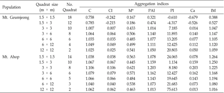
Table 2. Changes in gathering strength of Carex siderosticta at different sampling quadrat sizes
Population Quadrat size (m × m)
No.
Quadrat
Aggregation indices
C CI M* PAI PI Ca IM
Mt. Geumjeong 1.5 × 1.5 1.5 × 3 3 × 3 3 × 6 6 × 6 6 × 12
12 × 12
18 12 10 8 6 4 2
0.758 0.785 1.007 1.064 1.035 1.049 1.025
-0.242 -0.215 0.007 0.064 0.035 0.049 0.025
0.167 0.186 0.433 0.506 0.485 0.499 0.541
0.321 0.474 1.014 1.140 1.077 1.111 1.050
-0.610 -4.317 7.185 11.893 13.205 12.425 20.803
-0.679 -0.526 0.014 0.140 0.077 0.112 0.050
0.388 0.527 1.047 1.147 1.105 1.120 1.059
Mt. Ahop 1.5 × 1.5
1.5 × 3 3 × 3 3 × 6 6 × 6 6 × 12
12 × 12
14 10 8 6 5 3 2
1.038 1.067 1.106 1.079 1.066 1.040 1.062
0.038 0.067 0.106 0.079 0.066 0.040 0.062
0.563 0.445 0.621 0.571 0.484 0.538 0.463
1.078 1.159 1.203 1.162 1.143 1.073 1.013
24.065 1.134 8.180 12.427 19.645 21.683 75.613
0.078 0.159 0.203 0.162 0.143 0.073 0.013
1.264 1.250 1.225 1.168 1.194 1.080 1.016 example, in Sokal and Oden [19]. Thus, if an individual is
randomly distributed for class k, the normalized I (k) for the standard normal deviation (SND) for the plant genotype, g (k) = {I (k) - u1}/u21/2, asymptotically has a standard nor- mal distribution [6]. Hence, SND g(k) values exceeding 1.96, 2.58, and 3.27 are significant at the probability levels of 0.05, 0.01, and 0.001, respectively.
Results
The spatial pattern of individualsPopulation densities (D) varied from 0.547 to 5.778, with a mean of 2.644 (Table 1). The D value of Mt. Geumjeong area (3.108) is higher than Mt. Ahop area (2.180). There was shown significant difference between both mountain areas.
The values (R) of spatial distance (the rate of observed dis- tance-to-expected distance) among the nearest individuals were higher than 1 and the significant index of R (Cr) was
> 2.58. When this parameter was applied to two areas, the small plots (1.5 m × 1.5 m, 1.5 m × 3 m, 3 m × 3 m, and 3 m × 6 m) of C. siderosticta were uniformly distributed in the forest community (Table 1). However, C. siderosticta were aggregately distributed in large plots (6 m × 12 m, 12 m
× 12 m, and 12 m × 24 m) (Table 1).
The degree of population aggregation
Dispersion index (C) were higher than 1 except two quad- rats (1.5 m × 1.5 m and 1.5 m × 3 m for Mt. Geumjeong area) (Table 2). Thus aggregation indices (CI) were positive except two plots at Mt. Geumjeong which indicate a clump-
ed distribution. The mean crowding (M*) and patchiness in- dex (PAI) showed positive values. In Mt. Ahop, the three indices, C, M*, PAI were >1 and their values of PI and Ca except two plots were also shown greater than zero, thus it means aggregately distributed. The most individuals of C. siderosticta were clustered and the distribution pattern of the C. siderosticta was quadrat-sampling dependent. As the sizes of quadrat were greater, the PI values of C. siderosticta showed high.
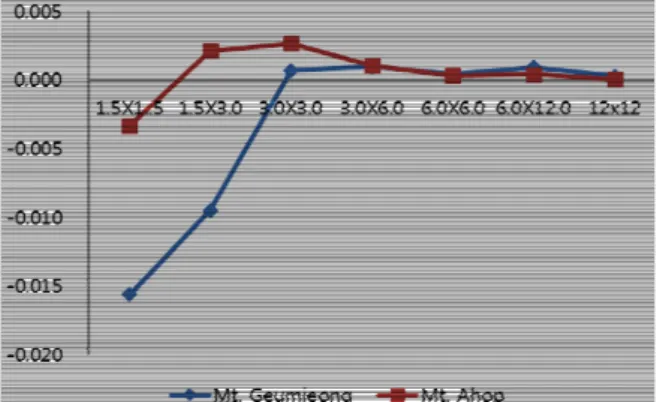
Morisita index (IM) is related to the patchiness index (PAI) and showed an overly steep slope at the plot 3 m x 3 m in Mt. Geumjeong and at the plot 1.5 m x 3 m in Mt.
Ahop. When the area was smaller than 1.5 m x 3 m, the degree of aggregation increased significantly with increasing quadrat sizes, while the patchiness indices did not change from the plot 6 m × 6 m to 12 m × 24 m.
The mean aggregation number (δ) analysis showed that the reasons for aggregation of C. siderosticta differed in quad- rats with different plot sizes. The most clusters at 25 quadrat was determined by environmental factors. When the size was one 2.5 m × 5 m plot at west, the cluster was determined by both species characteristics and environmental factors.
Analysis of spatial autocorrelation
The spatial autocoefficient, Moran's I is presented in Table 3. Separate counts for each type of joined individuals and for each distance class of separation were tested for sig- nificant deviation from random expectations by calculating the SND. Moran's I of C. siderosticta significantly differed from the expected value in only 16 of 40 cases (40%). Five
Table 3. Spatial autocorrelation coefficients (Moran's I) among two populations of Carex siderosticta for ten distance classes
Population I II III IV V VI VII VIII IX X
Mt. Geumjeong Mt. Ahop
0.449**
0.405
0.359* 0.347
0.333* 0.319
0.118 0.240
0.017 0.021
0.016 0.134
-0.103 -0.055
-0.148 0.023
-0.206 -0.162
-0.423 -0.553
*: p<0.05, **: p<0.01, ***: p<0.001.
Fig. 1. The curves of patchiness according to geographic dis- tances for two communities of Carex siderosticta using values of Green index. X axis is quadrat sizes (m × m).
Fig. 2. The changes of the mean aggregation numbers for com- munities of Carex siderosticta. X axis is quadrat sizes (m
× m).
of these values (31.3%) were negative, indicating a partial dissimilarity among pairs of individuals in the 10 distance classes. Eleven of the significant values (68.7%) were pos- itive, indicating similarity among individuals in the first 4 distance classes, i.e., pairs of individuals can separate by more than 10 m. Namely, significant aggregations were par- tially observed within IV classes. As a matter of course, the negative SND values at classes VI, VII, VIII, and X. Thus, dissimilarity among pairs of individuals could found by more than 15.5 m.
The comparison of Moran’s I values to a logistic re- gression indicated that a highly significant percentage of in- dividual dispersion in C. siderosticta populations at Mt.
Geumjeong could be explained by isolation by distance.
Discussion
When R = 1, it is a random distribution; R < 1, it is an aggregation; R > 1, it is a uniform distribution [14].
According to this rule, all plots and areas of C. siderosticta at Mt. Geumjeong are uniform distribution (Table 1).
However, According to dispersion indices of Llord [16], many plots are not uniform distribution (Table 2) and not consistent with the rule. R = rA/rB [5]. N for rA is total num- bers of within the plot and rB is concerned with plot size.
Although, a large plot has large N, the plot size is not N.
As D is the number of individuals per plot size, the nearest
neighbor rule by Clark and Evans [5] is good for spatial pattern. 16 plots (66.7%) showed were uniform distributed.
In only 8 plots (33.3%), the three indices, C, M*, PAI were
>1, and PI and Ca > 0, thus it means aggregately distributed.
Aggregation is mainly caused by the environmental factors [14]. When δ > 2, the aggregation was mainly caused by both species characteristics and environmental factors [14].
Most 23 plots except one had low δ < 2. I recognized that the important environmental factors might be considered competition, growth rate, little decomposition, light, and be- low-ground resources. The characteristics of the C. side- rosticta concerned included primarily their life history, artifi- cial disturbance, and population density. Life history theory seeks to understand the variation in traits such as growth rate, number and size of offspring and life span observed in nature, and to explain them as evolutionary adaptations to environmental conditions [22]. Artificial disturbances are important environmental factors affecting C. siderosticta such as constitutional roads at east area, temple construction at west area, and farming at south area. At the plots which had fewer C. siderosticta, the cluster was mainly determined by C. siderosticta themselves. Although the small proportion of seeds from mother removed by ants, 99% seeds in C. side- rosticta fell within 20 cm of the scape and 91% within 10 cm of the scape [12]. In addition, the mean value of the ag- gregation index changed irregularly with population growth rate [4].
A significant positive value of Moran's I indicated that pairs of individuals separated by distances that fell within distance class V had similar individuals, whereas a sig- nificant negative value indicated that they had dissimilar in- dividuals (Table 3). The overall significance of individual correlograms was tested using Bonferroni's criteria. The re- sults revealed that patchiness similarity was shared among individuals within up to a scale of a 7.5 m~10 m distance.
Thus it was looked for the presence of dispersion correla- tions between neighbors at this scale.
The results from this study are consistent with the suppo- sition that a plant population is subdivided into local demes, or neighborhoods of related individuals [7, 11]. Previous re- ports on the local distribution of genetic variability sug- gested that microenvironmental selection and limited gene flow are the main factors causing substructuring of alleles within a population [9].
In conclusion, C. siderosticta populations within Mt.
Geumjeong was observed a strong spatial structure. Neigh- boring patches of C. siderosticta are predominantly 7.5 m to 10 m apart on average. The present study demonstrates that a spatial structure of C. siderosticta in the Mt. Geumjeong populations could be explained by isolation by distance, lim- ited gene flow, and topography. However, if the natural populations were disturbed by human activities, the ag- gregation was occurred in more short distance than a scale of a 7.5 m~10 m distance. The results of this study were used as systematic conservation planning which is an effec- tive way to seek and identify efficient and effective types of reserve design to capture or sustain the highest priority biodiversity values and to work with communities in sup- port of local ecosystems. Conservation biology is an ob- jective science when biologists advocate for an inherent val- ue in nature.
References
1. Arbous, A. G. and Kerrich, J. E. 1951. Accident statistics and the concept of accident proneness. Biometrics 7, 340-342.
2. Bernard, J. M. 1990. Life history and vegetative reproduction in Carex. Can. J. Bot. 68, 1441-1448.
3. Borcard, D. and P. Legendre. 2012. Is the Mantel correlo- gram powerful enough to be useful in ecological analysis?
A simulation study. Ecology 93, 1473-1481.
4. Caswell1, H., Takenori Takada, T. and Hunte, C. M. 2004.
Sensitivity analysis of equilibrium in density-dependent ma- trix population models. Letters 7, 380-387.
5. Clark, P. J. and Evans, F. C. 1954. Distance to nearest neigh-
bor as a measure of spatial relationships in populations.
Ecology 35, 445-453.
6. Cliff, A. D. and Ord, J. K. 1971. Spatial autocorrelation. Pion, London.
7. Ehrlich, P. R. and Raven, P. H. 1969. Differentiation of populations. Science 165, 1228-1232.
8. Elith, J. and Burgman, M. A. 2002. Habitat models for PVA.
In: Brigham, C. A., Schwanz, M. W. (Eds.), Population Viabi- lity in Plants. Springer.
9. Epperson, B. K., Chung, M. G. and Telewski, F. W. 2003.
Spatial pattern variation in a contact zone of Pinus ponderosa and P. arizonica (Pinaceae). Am. J. Bot. 90, 25-31.
10. Evans, K. L., Duncan, R. P., Blackburn, T. M. and Crick, H. Q. P. 2005. Investigating geographic variation in clutch size using a natural experiment. Funct. Ecol. 19, 616-624.
11. Garnier, L. K. M., Durand, J. and Dajoz, I. 2002. Limited seed dispersal and microspatial population structure of an agamospermous grass of West African savannahs. Hyparrhe- nia diplandra (Poaceae). Am. J. Bot. 89, 1785-1791.
12. Guitián, P., Medrano, M. M. and Guitián, J. 2003. Seed dis- persal in Erythronium dens-canis L. (Liliaceae): variation among habitats in a myrmecochorous plant. Plant Ecology 169, 171-177.
13. Legendre, P. and Fortin, M. J. 1989. Spatial pattern and eco- logical analysis. Vegetatio 80, 107-138.
14. Lian, X., Jiang, Z., Ping, X., Tang, S., Bi, J. and Li, C. 2012.
Spatial distribution pattern of the steppe toad-headed lizard (Phrynocephalus frontalis) and its influencing factors. Asian Herpetol. Res. 3, 46-51.
15. Liebhold, A. M. and Gurevitch, J. 2002. Integrating the stat- istical analysis of spatial data in ecology. Ecography 25, 553-557.
16. Lloyd, M. 1967. Mean crowding. J. Ani. Ecol. 36, 1-30.
17. Peres-Neto, P. R., Legendre, P., Dray, S. and Borcard, D.
2006. Variation partitioning of species data matrices: estima- tion and comparison of fractions. Ecology 87, 2614-2625.
18. Scott, J. M., Heglund, P. J., Samson, F., Haufler, J., Morrison, M., Raphael, M. and Wall, B. 2002. Predicting Species Occurrences: Issues of Accuracy and Scale, pp. 868, Island Press, Covelo, CA.
19. Sokal, R. R. and Oden, N. L. 1978. Spatial autocorrelation in biology 1. Methodology. Biol. J. Linn. Soc. 10, 199-228.
20. Sokal, R. R. and Oden, N. L. 1978. Spatial autocorrelation in biology 2. Some biological implications and four applica- tions of evolutionary and ecological interest. Biol. J. Linn.
Soc. 10, 229-249.
21. Sone, K., Ohkubo, K., Matsuo, T. and Hata, K. 2013. Spatial distribution pattern of pine trees killed by pine wilt disease in a sparsely growing, young pine stand. J. Plant Stud. 2, 36-41.
22. Souza, A. F. and Martins, F. R. 2004. Microsite specialization and spatial distribution of Geonoma brevispatha, a clonal palm in south-eastern Brazil. Ecol. Res. 19, 521-532.
23. Yan-Cheng, T. and Qiu-Yun, X. 1989. Cytological studies of Carex siderosticta Hance (Cyperaceae) and its importance in phytogeography. Cathaya 1, 49-60.
초록:금정산과 아홉산의 대사초 집단의 공간적 분포 양상 허만규*
(동의대학교 분자생물학과)
식물 보존의 권고지역에서 식물 집단의 공간적 데이터는 여러 목적에서 중요하다. 부산광역시 금정산과 아홉산 의 대사초(Carex siderosticta)의 지리적 거리에 따른 공간적 분포를 분석하였다. 공간적 양상의 분석 방법은 여러 패치 척도, 분산 척도에 의거한 plot(플롯)의 크기에 따라 집단의 균질성 또는 운집을 분석하였다. 대사초의 많은 자연 플롯은 산림군락에서 균질하지 않았다. 예를 들면 균질한 플롯은 6.0 m × 6.0 m 이내였다. 플롯의 크기가 6.0 m × 12.0 m 이상이면 운집되었다. 대사초의 이웃 패치는 평균 7.5 m에서 9.0 m사이였다. 그런데 자연집단이 인간의 활동에 의해 교란되면 운집은 9.0 m보다 짧은 거리에서 일어났다. 결론적으로 대사초의 지리적 분포는 플롯의 밀도에 균질하지 않았고 금정산과 아홉산 집단에서 집단 크기에 따라 다르며 인간의 간섭은 플롯에서 밀 도 효과를 일으킨다.