Switching properties of CUSUM charts for controlling mean vector

Switching properties of CUSUM charts for controlling mean vector ^†

Duk-Joon Chang ¹ · Sunyeong Heo ²

12 Department of Statistics, Changwon National University

Received 30 June 2012, revised 21 July 2012, accepted 24 July 2012

Abstract

Some switching properties of multivariate control charts are investigated when the interval between two consecutive sample selections is not fixed but changes according to the result of the previous sample observation. Many articles showed that the perfor- mances of variable sampling interval control charts are more efficient than those of fixed sampling interval control charts in terms of average run length (ARL) and average time to signal (ATS). Unfortunately, the ARL and the ATS do not provide any information on how frequent a switch is being made. We evaluate several switching properties of two sampling interval Shewhart and CUSUM procedures for controlling mean vector of correlated quality variables.

Keywords: Average number of switches to signal, average sampling interval, probability of switch.

1. Introduction

The purpose of a control chart is to detect assignable causes of variation so that these causes can be found and eliminated. During the control process, one wishes to detect any departure from a satisfactory state as quickly as possible and identify which attributes are responsible for the deviation. Thus, a good control chart detects shifts quickly in the process when the process is out-of-control state, and produces few false alarms when the process is in-control state.

Many situations in industrial quality control involve a vector of measurements of two or more related quality variables rather than a single quality variable. When the quality variables are correlated, one could obtain better sensitivity by using multivariate control procedures than separate control variables for each of the quality variables.

Traditional sampling practice in using a control chart is to take samples from the process at fixed sampling interval (FSI) and performances of control charts have been developed when the sampling interval between samples is fixed. In recent years, application of variable

† This research is financially supported by Changwon National University in 2011-2012.

1

Professor, Department of Statistics, Changwon National University, Changwon 641-773, Korea.

2

Corresponding author: Associate professor, Department of Statistics, Changwon National University,

Changwon 641-773, Korea. E-mail: [email protected]

sampling interval (VSI) control charts has become quite frequent and several articles have been published about them in which the sampling interval is varied as a function of what is observed from the process. The basic idea of VSI control chart is that the time interval should be short if there is some indication of a process change and should be long if there is no indication of a process change. If the indication of a process change is strong enough, then the VSI chart signals in the same way as the FSI control chart. Therefore, the idea of VSI procedure is intuitively reasonable.

VSI procedures for controlling the amount of dissolved oxygen in streams were first investi- gated by Arnold (1970). Extensions of Arnold’s work was presented by Smeach and Jernigan (1977). Reynolds and Arnold (1989) developed general expressions for performances of a VSI Shewhart chart such as the ARL and ATS when the process is in control and when it is out of control. Multivariate control charts with VSI scheme were studied by Cho (2010), Im and Cho (2009), Chang and Heo (2006).

One shortcoming in applying VSI procedure is that frequent switching between different sampling intervals requires more cost and effort to administer the process than correspond- ing FSI scheme. Amin and Letsinger (1991) described general procedures for VSI scheme and examined switching behavior and runs rules for switching between different sampling intervals on univariate ¯ X -chart. They also presented that the average number of switches to signal (ANSW) of the CUSUM and EWMA procedures exists far fewer than the Shewhart procedure. Amin and Hemasinha (1993) presented expressions for the ANSW and ATS for VSI ¯ X -chart with runs rules for evaluating the switching behavior.

In this paper, we evaluated various switching properties of two sampling interval multi- variate Shewhart and CUSUM control charts for controlling mean vector of multivariate normal process N p (µ, Σ).

2. Description of the considered control procedures

Suppose that the production process of interest has p quality variables whose distribution is multivariate normal with mean vector µ and variance-covariance matrix Σ. At each sampling occasion i (i = 1, 2, · · · ), we take a sequence of samples for each quality variables of size n from the production process where the observations within and between samples are assumed to be independent. We also assume that (µ ₀ , Σ 0 ) be the known target process values for (µ, Σ). Then the joint density function of all observations is given by

1 (2π) ^np/2 

Σ  

n/2 exp[− 1

2 (X − µ) ⁰ Σ ⁻¹ (X − µ)].

Because a control chart can be viewed as repeated tests of significance, we can obtain multivariate control statistic by using the likelihood ratio test (LRT) statistic for testing H 0 : µ = µ ₀ where target dispersion matrix Σ 0 is known. Then the likelihood ratio λ at the i th sample can be expressed as

λ = exp

"

− n

2 ( ¯ X _i − µ) ⁰ Σ ⁻¹ ₀ ( ¯ X _i − µ)

#

. (2.1)

Let Z _i ² be −2lnλ. Then

Z _i ² = n( ¯ X _i − µ) ⁰ Σ ⁻¹ ₀ ( ¯ X _i − µ). (2.2) The null hypothesis will be rejected if Z _i ² ≥ χ ² _1−α (p). Thus, the LRT statistic Z _i ² under H ₀ : µ = µ

0 can be used as the control statistic for monitoring mean vector of p related quality variables.

A FSI multivariate Shewhart chart for µ based on the LRT statistic signals whenever Z _i ² ≥ h S . For two sampling interval multivariate Shewhart chart, suppose that the short sampling interval d 1 is used when Z _i ² ∈ (g S , h S ] and the long sampling interval d 2 is used when Z _i ² ∈ (0, g S ] where d 1 < d 2 . Thus, g S is the boundary between the regions specifying d 1 and d 2 .

If the process is in-control, the control statistic Z _i ² has a chi-squared distribution with p degrees of freedom when µ = µ

0 and Σ = Σ ₀ . For arbitrary values of µ, Z _i ² has a non central chi-squared distribution with p degrees of freedom and noncentrality parameter τ ² = n(µ − µ ₀ ) ⁰ Σ ⁻¹ ₀ (µ − µ ₀ ). Chengular-Smith et al. (1989) worked on the VSI Shewhart control charts for mean vector.

Therefore, the percentage point of Z _i ² can be obtained from the chi-square distribution when the process is in-control or target mean vector has changed. The value h _S can be obtained from chi-square distributions to satisfy a desired ARL. And, ARL of this chart can be calculated as 1/P (signals) where P (signals) denotes the probability that χ ² exceeds the h _S . The on-target ARL based on P (signals) is determined from the probability that χ ² exceeds the h _S under the central χ ² (p) distribution while the off-target ARL based on P (signals) is determined from the probability that χ ² exceeds the upper control limit (UCL) under the noncentral χ ² (p) distribution

A FSI multivariate CUSUM chart based on LRT statisic Z _i ² (i = 1, 2, · · · ) can be con- structed as

Y i = max {Y i−1 , 0} + (Z _i ² − k), (2.3) where the starting value Y ₀ is a specified constant which is frequently chosen to be zero, and reference value k (k ≥ 0). This chart signals whenever Y _i ≥ h C where h _C is UCL of the CUSUM chart. For two sampling interval multivariate CUSUM chart, suppose that the short sampling interval d ₁ is used when Y _i ∈ (−k, g _C ] and the long sampling interval d ₂ is used when Y i ∈ (g C , h C ] where d 1 < d 2 . Thus, g S is the boundary between the regions specifying d 1 and d 2 . When the process is in-control or mean vector µ has changed, the ARL and ATS performances of the CUSUM chart in (2.3) and the design parameters g C and h C

can be obtained by Markov chain approach. Markov chain approach for EWMA chart can be referred from Chang et al. (2003).

3. Properties of VSI procedures

A control chart is maintained by taking samples from the process and plotting in time

order on the chart some control statistic which is a function of the samples. The operation

of a control chart in detecting process changes can be described simply in terms of a control

statistic and two disjoint regions, the signal region and the in-control region. In each case,

the control statistic is compared with the control limits and if the control statistic falls

within the control limits, the process is assumed to be in-control and allowed to continue for the next sample. On the other hand, if a control statistic falls outside the control limits, the chart then signals and rectifying action is needed to identify the cause of changes and bring the process back into in-control state.

One traditional practice in using a control chart is to take samples from the process at FSI and properties of control charts have been developed when the sampling interval between samples is fixed. The basic idea of VSI control chart is that the time interval should be short if there is some indication of a process change and should be long if there is no indication of a process change. If the indication of a process change is strong enough, then the VSI chart signals in the same way as the FSI control chart. For VSI chart, the sampling times are random variables and the sampling interval depends on the past sample informations of X ₁ , X ₂ , · · · , X _i .

To implement two sampling interval control charts, the in-control region is divided into 2 regions I ₁ , I ₂ where I _i is the region in which the sampling interval d _i is used (i = 1, 2).

In this paper, we assume that the two sampling interval chart is started at time 0 and the interval used before the first sample, is a fixed constant, say d ₀ . Then the ARL and ATS can be expressed as

( ARL = 1 + ψ ₁ + ψ ₂ AT S = d 0 + d 1 ψ 1 + d 2 ψ 2

(3.1)

where ψ i is the expected number of samples before the signal. Then the ATS can be reex- pressed as AT S = d·ARL and d can be interpreted as the average sampling interval (ASI) of the chart to signal, and ρ 1 can be considered as the long-run proportion of sampling interval that d 1 is used where

d = d ₁ ρ ₁ + d ₂ (1 − ρ ₁ ) and ρ ₁ =

( (ψ ₁ + 1)/ARL if d ₀ = d ₁ ψ 1 /ARL if d 0 = d 2 .

Through theoretical and numerical comparisons between FSI and VSI procedures, many researchers evaluated that VSI schemes are substantially more efficient than FSI schemes in terms of ARL and ATS. But, the ARL and the ATS do not provide any switching information on different sampling intervals of VSI schemes. Hence, it is necessary to define the number of switches (NSW) as the number of switches made from the start of the process until the chart signals, and let ANSW be the expected value of the NSW. The ANSW can be obtained by using Wald’s identity as follows

AN SW = ARL · P (switch) (3.2)

where the ARL can be approximated by a Markov chain approach for the multivariate CUSUM procedures, and central or noncentral χ ² (p) distribution for multivariate Shewhart chart, and is equal to 1/P (signal). And, the probability of switch is given by

P (switch) = P (d 1 ) · P (d 2 |d 1 ) + P (d 2 ) · P (d 1 |d 2 ) (3.3)

where P (d _i ) is the probability of using sampling interval d _i , and P (d _i |d j ) is the conditional

probability of using sampling interval d _i in the current sample given that the sampling

interval d _j (d _i 6= d _j ) was used in the previous sample. Amin and Lestinger (1991) defined the number of samples to switch (NSSW) as the number of samples taken from the time the process starts using the sampling interval d i until a switch is made to sampling interval d j

(i 6= j), and they also defined the average number of samples until a switch (ANSSW) as the expected value of the number of samples until a switch. The number of samples until a switch occurred has a geometric distribution with parameter P (switch) when the process doesn’t change. Thus the ANSSW is as follows

AN SSW = 1

P (switch) , P (switch) > 0, (3.4) For comparing the efficiencies of the considered charts, we also evaluated P (d i → d j ) as the probability of a switch from d i to d j (d i 6= d j ) of proposed two sampling interval multivariate Shewhart and CUSUM procedures.

4. Concluding remarks

In evaluating the properties of the VSI structure, it is usual to compare the performances of the VSI procedure to the same procedure using fixed sampling intervals. The process parameters are selected for both FSI and VSI control scheme having the same in control ARL and ATS values since the ASI is equal to one unit.

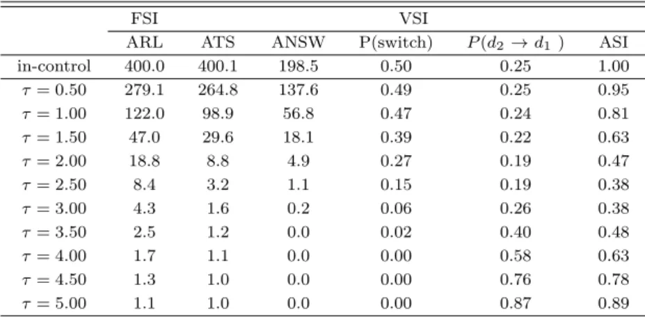
In our computation, each scheme was calibrated so that the on-target ARL was approxi- mately equal to 400.0 and the sample size for each characteristic was five for p = 3 and p = 5, and we used d 0 = 1.0, d 1 = 0.1, d 2 = 1.9. For convenience we let that target mean vector µ 0 = 0, and all diagonal elements σ _r0 ² in Σ 0 is 1.0 and off-diagonal elements in Σ 0 is 0.3, respectively. It is also assumed that the shift from target value µ

0 to arbitrary value µ occurs as soon as a sample is taken. ANSW, P (switch) and P (d 2 → d 1 ) of CUSUM procedures are obtained by simulation with 10,000 iterations.

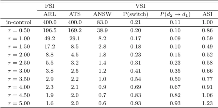
Numerical results in Table 4.1 through Table 4.4 show that the VSI procedures are far superior to the corresponding FSI control procedures in terms of ATS. And, it can also be seen that the performance of the CUSUM procedures is more efficient than those of Shewhart procedures for small or moderate shifts of the process mean vector.

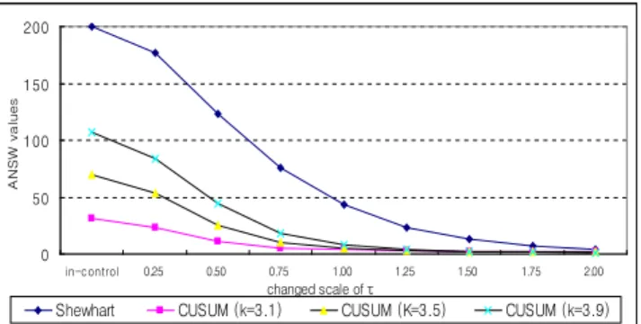
In this paper, we mainly focused on switching information on different sampling intervals of VSI schemes. From the results in Table 4.2 through Table 4.4, we found that multivariate CUSUM chart with smaller reference value k results in fewer switches between the two sampling intervals. It can be seen that the CUSUM procedures has substantially fewer switches when compared to the Shewhart procedure for small or moderate changes of the mean vector.

For small or moderate changes of the process, P (switch) of CUSUM chart is consider-

ably smaller than Shewhart chart’s one, and as k increases P (switch) of CUSUM chart is

gradually increasing. However, when the shift is large, P (switch) of Shewhart chart becomes

remarkably smaller. The results of Table 4.1 and Figure 4.3 show that for moderate changes,

ASI values of Shewhart have a tendency to be lower than CUSUM charts’s ones. In addi-

tion, when the sample interval changes from d 1 to d 2 , as the amount of process shift becomes

larger, the probability in CUSUM chart increases a little, but the probability in Shewhart

chart is declining slightly and then increasing after noncentral parameter τ ² = 2.0 ² . Figure

4.2 shows the same result.

Generally, when one is more interested in detecting a small amount of process shift, CUSUM chart with smaller values of k will be recommended not only in the respect of ATS but also in the switching performance. The optimal selection of reference value k in VSI multivariate CUSUM procedure is influenced by the size of the shift in the mean vector not only for being detected quickly but also in the respect of switching property.

0 50 100 150 200

in-control 0.25 0.50 0.75 1.00 1.25 1.50 1.75 2.00

changed scale of τ

ANSW values

Shewhart CUSUM (k=3.1) CUSUM (K=3.5) CUSUM (k=3.9)

Figure 4.1 ANSW performances of the charts (p =3)

0.0 0.2 0.4 0.6 0.8 1.0

in- control

0.5 1.0 1.5 2.0 2.5 3.0 3.5 4.0 4.5 5.0

changed scale of τ

Prob(d2 → d1)

Shewhart CUSUM (k=3.1) CUSUM (K=3.5) CUSUM (k=3.9)

Figure 4.2 P (d

→ d

) performances of the charts (p =3)

0.0 0.2 0.4 0.6 0.8 1.0

in- control

0.5 1.0 1.5 2.0 2.5 3.0 3.5 4.0 4.5 5.0

changed scale of τ

ASI values .

Shewhart CUSUM (k=3.1) CUSUM (K=3.5) CUSUM (k=3.9)

Figure 4.3 ASI performances of the charts (p =3)

Table 4.1 Numerical performances of multivariate Shewhart chart (p = 5)

FSI VSI

ARL ATS ANSW P(switch) P (d

→ d

) ASI

in-control 400.0 400.1 198.5 0.50 0.25 1.00

τ = 0.50 279.1 264.8 137.6 0.49 0.25 0.95

τ = 1.00 122.0 98.9 56.8 0.47 0.24 0.81

τ = 1.50 47.0 29.6 18.1 0.39 0.22 0.63

τ = 2.00 18.8 8.8 4.9 0.27 0.19 0.47

τ = 2.50 8.4 3.2 1.1 0.15 0.19 0.38

τ = 3.00 4.3 1.6 0.2 0.06 0.26 0.38

τ = 3.50 2.5 1.2 0.0 0.02 0.40 0.48

τ = 4.00 1.7 1.1 0.0 0.00 0.58 0.63

τ = 4.50 1.3 1.0 0.0 0.00 0.76 0.78

τ = 5.00 1.1 1.0 0.0 0.00 0.87 0.89

Table 4.2 Numerical performances of multivariate CUSUM chart (p = 5, k = 5.2)

FSI VSI

ARL ATS ANSW P(switch) P (d

→ d

) ASI

in-control 400.0 400.0 37.8 0.09 0.05 1.00

τ = 0.50 172.3 138.3 15.5 0.09 0.05 0.80

τ = 1.00 49.3 29.8 4.5 0.09 0.05 0.61

τ = 1.50 21.5 12.5 2.6 0.13 0.07 0.58

τ = 2.00 12.1 7.2 2.0 0.18 0.10 0.59

τ = 2.50 7.9 4.8 1.8 0.26 0.15 0.62

τ = 3.00 7.6 3.6 1.5 0.33 0.22 0.48

τ = 3.50 4.2 2.9 1.3 0.42 0.31 0.69

τ = 4.00 3.3 2.5 1.2 0.51 0.43 0.75

τ = 4.50 2.7 2.2 1.1 0.62 0.57 0.82

τ = 5.00 2.3 2.1 1.0 0.75 0.72 0.91

Table 4.3 Numerical performances of multivariate CUSUM chart (p = 5, k = 5.5)

FSI VSI

ARL ATS ANSW P(switch) P (d

→ d

) ASI

in-control 400.0 400.0 60.8 0.15 0.08 1.00

τ = 0.50 183.5 152.9 26.5 0.15 0.07 0.83

τ = 1.00 46.8 26.9 5.9 0.13 0.07 0.58

τ = 1.50 18.2 9.4 2.6 0.15 0.09 0.52

τ = 2.00 9.8 5.2 1.9 0.21 0.13 0.53

τ = 2.50 6.2 3.6 1.5 0.29 0.20 0.58

τ = 3.00 4.4 2.8 1.3 0.37 0.30 0.64

τ = 3.50 3.3 2.4 1.1 0.48 0.43 0.72

τ = 4.00 2.6 2.2 1.0 0.61 0.58 0.83

τ = 4.50 2.2 2.1 0.9 0.76 0.74 0.94

τ = 5.00 1.8 2.0 0.7 0.88 0.88 1.09

Table 4.4 Numerical performances of multivariate CUSUM chart (p = 5, k = 5.8)

FSI VSI

ARL ATS ANSW P(switch) P (d

→ d

) ASI

in-control 400.0 400.0 83.0 0.21 0.11 1.00

τ = 0.50 196.5 169.2 38.9 0.20 0.10 0.86

τ = 1.00 49.2 29.1 8.2 0.17 0.09 0.59

τ = 1.50 17.2 8.5 2.8 0.18 0.10 0.49

τ = 2.00 8.8 4.5 1.8 0.23 0.15 0.52

τ = 2.50 5.5 3.2 1.4 0.31 0.23 0.58

τ = 3.00 3.8 2.5 1.2 0.41 0.35 0.66

τ = 3.50 2.9 2.2 1.0 0.54 0.50 0.77

τ = 4.00 2.3 2.1 0.9 0.69 0.67 0.91

τ = 4.50 1.9 2.0 0.7 0.83 0.82 1.06

τ = 5.00 1.6 2.0 0.6 0.93 0.93 1.23

References

Amin, R. W. and Hemasinha, R. (1993). The switching behavior of ¯ X charts with variable sampling intervals.

Communications in Statistics - Theory and Methods, 22, 2081-2102.

Amin, R. W. and Letsinger. W. C. (1991). Improved swiching rules in control procedures using variable sampling intervals. Communications in Statistics - Simulation and Computation, 20, 205-230.

Arnold, J. C. (1970). A Markovian sampling policy applied to quality monitoring of streams. Biomerics, 26, 739-747.

Bai, D. S. and Lee, K. T. (2002). Variable sampling interval ¯ X control charts with an improved switching rule. International Journal of Production Economics, 76, 189-199.

Chang, D. J. and Heo, S. (2006). Performances of VSI multivariate control charts with accumulate-combine approach. Journal of the Korean Data & Information Science Society, 17, 973-982.

Chang, D. J., Kwon, Y. M. and Hong, Y. W. (2003). Markovian EWMA control chart for several correlated quality characteristics. Journal of the Korean Data & Information Science Society, 14, 1045-1053.

Chengular-Smith, I. N., Arnold, J. C. and Reynolds, M. R., Jr. (1989). Variable sampling intervals for multiparameter Shewhart charts. Communications in Statistics - Theory and Methods, 18, 1769-1792.

Cho, G. Y. (2010). Multivariate Shewhart control charts with variable sampling intervals. Journal of the Korean Data & Information Science Society, 21, 999-1008.

Im, C. D. and Cho, G. Y. (2009). Multiparameter CUSUM charts with variable sampling intervals. Journal of the Korean Data & Information Science Society, 20, 593-599.

Reynolds, M. R., Jr. and Arnold, J. C. (1989). Optimal one-sided Shewhart control charts with variable sampling intervals between samples. Sequential Analysis, 8, 51-77.

Ryu, J. H. and Wan, H. (2010). Optimal design of a CUSUM chart for a mean shift of unknown size. Journal of Quality Technology, 42, 311-326.

Smeach, S. C. and Jernigan, R. W. (1977). Further aspect of a Markovian sampling policy for water quality

monitoring. Biometrics, 33, 41-46.