Urbanization and Quality of Stormwater Runoff: Remote Sensing Measurements of Land Cover in an Arid City

1. Introduction

In cities, runoff from storms is widely known to degrade water quality by altering delicate hydrological patterns in the following ways: accelerated flow, disturbed ecological habitats, and increased load and concentrations of waterborne pollutants (USEPA,

2000). Urbanization can exacerbate these problems by increasing the total area of impervious surface over which stormwater flows, and urban landscapes are characterized by complex spatial heterogeneity including differ land uses and land covers (Wu et al., 2011). Research has repeatedly demonstrated that there is a strong positive relationship between the extent of

Urbanization and Quality of Stormwater Runoff:

Remote Sensing Measurements of Land Cover in an Arid City

Min Jo Kang*

, Victor Mesev* and Soe W. Myint**

*Department of Geography, Florida State University

**School of Geographical Sciences and Urban Planning, Arizona State University

Abstract : The intensity of stormwater runoff is particularly acute across cities located in arid climates.

During flash floods loose sediment and pollutants are typically transported across sun-hardened surfaces contributing to widespread degradation of water quality. Rapid, dense urbanization exacerbates the problem by creating continuous areas of impervious surfaces, perforated only by a few green patches. Our work demonstrates how the latest techniques in remote sensing can be used to routinely measure urban land cover types, impervious cover, and vegetated areas. In addition, multiple regression models can then infer relationships between urban land use and land cover types with stormwater quality data, initially sampled at discrete monitoring sites, and then extrapolated annually across an arid city; in our case, the city of Phoenix in Arizona, USA. Results reveal that from 30 storm event samples, solids and heavy metal pollutants were found to be highly related with general impervious surfaces; in particular, with industrial and commercial land use types. Repercussions stemming from this work include support for public policies that advocate environmental sustainability and the more recent focus on urban livability. Also, advocacy for new urban construction and re-development that both steer away from vast unbroken impervious surfaces, in place of more fragmented landscapes that harmonize built and green spaces.

Key Words : Stormwater runoff, Spectral Mixture Analysis (SMA), Water quality, Urbanization, Land use, Imperviousness

Received May 31, 2014; Revised June 9, 2014, Revised June 25, 2014; Accepted June 25, 2014.

†

Corresponding Author: Min Jo Kang ([email protected])

This is an Open-Access article distributed under the terms of the Creative Commons Attribution Non-Commercial License

(http://creativecommons. org/licenses/by-nc/3.0) which permits unrestricted non-commercial use, distribution, and reproduction in

any medium, provided the original work is properly cited

imperviousness and the volume of urban stormwater runoff; as well as a strong negative relationship between the area of imperviousness and stormwater quality (inter alia Arnold and Gibbons, 1996; Adams and Papa, 2000; Brabec et al., 2002; Tong and Chen, 2002; Lee and Heaney, 2003; Dougherty et al., 2004;

Carlson, 2008). Another consensus view is that predominantly flat impervious surfaces increase the amount of time that rainfall remains on the surface as runoff and reduces the rate of infiltration into the soil (USEPA, 2003). In addition to pollutants, such as oil, solvents, solids and heavy metals carried by stormwater runoff, studies have further demonstrated that discharges from storm drain systems often include waste and wastewater from non-point sources, referred to as illicit discharges. This results in untreated discharges contributing to elevated overall loads of organic and inorganic pollutants and pathogens (Lopes et al., 1994; UESPA, 2000; Brezonik and Stadelmann, 2002; Brattebo and Booth, 2003; Gobel et al., 2007;

Carlson, 2008). The link between widespread impervious surfaces_which tend to increase surface stormwater runoff and degrade the quality of water_is now widely established in the literature. What is also recognized is that rapid urbanization leads to more urban land being used for residential, commercial and industrial activities, and conversely fewer and smaller biophysical spaces (natural and undeveloped land composed mostly of vegetation and exposed soil) (Simon et al., 2009; Xiao et al., 2012). Commercial and industrial land use types tend to be more likely sources of pollutants than biophysical spaces, while low density residential land uses are less likely _ despite the widespread use of lawn fertilizers in many suburbs.

Particularly, key urban sources of heavy metal include building roofs, pavements, road dusts, agricultural support industries, chemical and associated produce manufacturing, commercial livestock processing industries, metal product manufacturing, meter processing manufacturing, motor vehicle service

facilities, and catchment soil quality, etc (Davis et al., 2001; Kennedy and Sutherland 2008; Wicke et al., 2012).

However, where more research is still required is on techniques that measure surface imperviousness quickly, more precisely and not by rigid categorical land use distinctions but on a sliding scale of imperviousness. To attempt this more continuous representation of urban imperviousness consider ground-based surveys, published maps and aerial photographs, which have traditionally been used to delineate land use and land cover types. These sources are collected sporadically, can be expensive and demand skilled manual interpretation. As a viable alternative, multispectral data captured by satellite remote sensors are a rapid and relatively cheaper means with which to not only calculate graded mixtures of impervious and biophysical land surfaces across the whole urban area (Liu et al., 2010) but also contribute to landscape ecology identification and landscape pattern analysis (Shao and Wu, 2008). In addition, Kim et al. (2013) applied hydrological modeling using high resolution multi-satellite precipitation analysis.

Moreover, satellite sensor images are digital and can

be analyzed using a variety of statistical methods. One

suite of calculations relies on spectral mixture models,

used widely by geospatial scientists to estimate

continuous ranges of land cover variability in the urban

landscape given known pure classes (Wu and Murray,

2003; Myint and Okin, 2009). Spectral Mixture

Analysis (SMA) models have been used to derive the

fractional contribution of endmember materials to

image spectra and monitor urban environments of

measuring water quality (Weng, 2012) and to classify

forest area in more detailed spatial scale (Song et al.,

2014). Additionally, Multiple Endmember Spectral

Mixture Analysis (MESMA) is constructed an

endmembers from candidate image and reference

endmembers as considering all combinations of library

endmembers of SMA model for the best-fit model

(Powell et al., 2007). Different approaches using spectral, spatial and temporal variability have been used to drive soft classification such as fuzzy theory and other sub-pixel mapping (Weng, 2010). In addition, the normalized difference vegetation index (NDVI) is a simple yet robust metric that calculates the abundance of chlorophyll in growing vegetation (Jiang et al., 2006) and characterize patterns of variation in time series data and track changes in vegetation cover (Jung and Change, 2013). Together these techniques can routinely, at high levels of accuracy and precision, measure pure and subtle combinations of impervious and biophysical surfaces. Such output is critical in calculating, with any degree of scientific rigor, the precise relationship between imperviousness and stormwater quality using inferential statistics, such as multiple regression models. Indeed the use of remote sensing, geographic information systems (GIS) and spatial statistics for measuring urbanization and urban hydrological interruptions is gaining momentum with researchers (Cruise et al., 2010).

Applications using medium spatial resolution data from Landsat TM satellite sensors are reported by Carlson (2004) while high spatial resolution sensors onboard the satellites IKONOS and QuickBird were investigated by Goetz et al. (2003) and Thanapura et al. (2007) respectively. Ganbaatar and Lee (2014) refined the spatial characteristics of crop lands using Landsat TM. Furthermore, laser-based LiDAR (light detection and ranging) data are an exciting new development that allows even finer precision for measuring detention basins (Liu and Wang, 2008;

Bailang et al,. 2010; Shin et al., 2014). Once measured by remote sensing, GIS and spatial statistics are critical for the rigorous analysis of how urban surfaces affect water flow and quality (see early work by Coroza et al., 1997 and a review by Martin et al., 2005). Most research focus on linear relationships (for example, Thanapura et al., 2007; Jat et al., 2009), but some develop stochastic modifications (see Adams and Papa,

2000), and even simulated flow (Tong and Shen, 2002).

In sum, remote sensing is quickly establishing a major role for collecting objective and current data on urban land use and urban land cover. These data are then analyzed to measure mixtures of impervious and biophysical (mostly vegetation and soil) surfaces that can be used to represent any city, but cities in arid areas are particularly prone to flash floods and frequent stormwater activity. One such arid city is Phoenix in the US state of Arizona, which is used as a test site to statistically explore the degree to which topographic factors _ surface imperviousness, vegetation coverage and drainage basin areas _ affect the levels of pollutant loads suspended in stormwater across an entire desert city. For dry-weather stormwater drainage planning, preparing for periodic drought and resultant strict water conservation and reuse are all critical factors (Pitt and Clark, 2008). In doing so, broader planning implications are explored for deciding on the types, quantities, spatial configuration and densities of construction, road paving and green space that may be developed in an arid city with respect to how these zones impact on the discharge and quality of stormwater. There seems to be a dearth of this type of research on cities located in the world’s arid zones. One notable contribution is of Nouh and Al-Noman (2009) who used applied regression models for the prediction of stormwater water quality in conjunction with dust storms in the Middle East.

We end with a discussion on the debate of how rapid and dense urban over-development can result in vast tracts of continuous impervious surfaces and hence exacerbate the runoff problem in a desert city. Also, how policies that advocate mixed land uses perforated by biophysical spaces are likely to lead to more reduced dispersion of water-borne pollutants.

These echo the recommendations of Thurston et al.

(2003) who advocate a ‘tradable allowance’ for

impervious surfaces; Brattebo and Booth (2003),

Conway (2007), and Schiff and Benoit (2007) on the

balance between quality and quantity of ‘permeable pavements;’ and even Carter and Jackson (2007) and Butler and Davis (2011) on more vegetated roofs. The debate can be widened to incorporate notions of environmental sustainability and urban livability; both underscored by ecological analogies of the ‘extended metabolism model,’ which balances resource inputs with waste outputs (Newman, 1999; Slavin, 2011), and the ‘carrying capacity,’ which is the population that a given habitat can support (Wedding and Crawford- Brown, 2007). Ultimately, the search is for a balance between quality of life, environmental habitat tolerance and economic progress (van Kamp et al., 2003). But for now the general consensus is on heterogeneous land use zoning policies, fragmented impervious surfaces interspersed with green patches, and a curb on expanding residential lot sizes (Stone and Bullen, 2006).

2. Study Area and Data

The Arizona city of Phoenix is one of the fastest growing in the United States. From approximately

100,000 in 1950 it grew to just under one million by 1990 and to 1.45 by 2010 on 474 square miles (US Census Bureau, 2010) (Fig. 1). Phoenix is an example of an urban area located in a warm and arid climatic zone where temperatures frequently exceed 38°C and the mean annual precipitation is typically between 16 and 20 cm, yet its proximity to elevated terrain contributes to some topographic heterogeneity. Indeed, the anomalous ridge pattern of Arizona’s mountains is partly responsible for severe storms in the central part of the state, as well as dust storms throughout Arizona.

For Phoenix this produces rainfall patterns that are typically variable with localized thunderstorms during the summer months producing flash floods and substantial runoff. Conversely, winter storms, which may last longer, are normally at lower intensities.

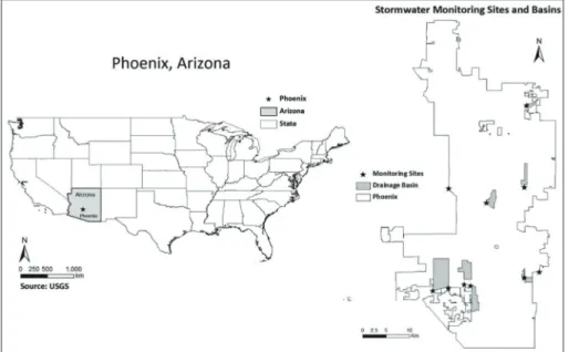
The City of Phoenix has seven outfall stormwater monitoring sites by the Flood Control District of Maricopa County (FCDMC) and are composed of seven outfall locations (discharges from a sewer, drain or stream) (Fig. 1). The outfall locations measure stormwater pollutant concentrations; a storm event is defined as more than 0.1 inches of rainfall occurring during at least 72 hours after the previous storm event

Fig. 1. Study Area: Phoenix, Arizona.

(City of Phoenix, 2005). Our analyses are based on storm event datasets and measures individual stormwater pollutant concentrations for the city. Data on stormwater pollutant concentrations are derived from 30 samples taken from the ten outfall locations between July 2002 and June 2007, and include biochemical oxygen demand (BOD

), total dissolved solids (TDS), total suspended solids (TSS), phosphorus, and oil and grease (all measured in mg/L);

and copper (Cu), zinc (Zn), and lead (Pb) (all measured in μg/l). Additionally, each storm event data includes land use data: acre size of industrial, commercial, residential, and undeveloped area. We calculated the percentage of various land use types based on acre sizes of each land use and drainage basins. The analysis is limited to the three in stream and seven outfall sites, which means that some hydrological basins are not directly monitored. Although a relatively small number of samples the ten sites are well distributed across the city, and in terms of land use and land cover, two of the seven outfall sites are located on industrial land, two on commercial, and one each for residential, agricultural and undeveloped.

In addition to data on stormwater quality, a remotely sensed image taken by the Landsat-5 Thematic Mapper (TM) satellite sensor on March 8, 2005 is used to measure the impervious and biophysical surfaces of Phoenix (Fig. 1). Landsat TM images offer global coverage, are sampled at a 30 m spatial resolution, and are routinely classified for many applications into broad land use and land cover categories, such as urban, commercial, residential, vegetation, etc. Their capacity to represent surface properties at multiple spectral wavelengths, including a thermal range, allows techniques such as spectral mixture analysis and the normalized difference vegetation index (NDVI) to measure mixtures of imperviousness and vegetation cover. However, medium spatial resolution remotely sensed data, such as those recorded by the Landsat TM sensor typically result in low classification accuracies

when used to interpret the complex arrangement of heterogeneous land cover types that are characteristic of urban areas. Slightly finer spatial resolutions, for example using 10 m data from SPOT sensors (see early work by Morgan et al., 1993), can improve classification accuracy, but only over the last decade have imagery at scales of a few meters or even sub meter resolutions been able to represent spatially distinct urban detail. However these finer spatial resolution images are data-heavy, require matching of multiple scenes to capture the entire city, and in any case contain excessive spectral noise which ultimately renders classification accuracies almost as low. Even finer spatial resolutions, associated with light detection and ranging (LiDAR) data, are also excellent at delineating topographic depressions in watersheds (Liu and Wang, 2008), but such surface variations at micro scales are not normally known to alter stormwater runoff patterns.

Instead the data we use from the Landsat TM multispectral sensor are more suited for calculating the entire range of impervious and biophysical surfaces across an entire city. We follow Carlson (2004) lead in using Landsat TM sensor data in conjunction with runoff measurements and an urban growth model to estimate impacts on future water quality.

However, we also investigate individual water

pollutants (solids and heavy metals) with respect to a

broader range of explanatory variables using inferential

models. Moreover, we use a fine spatial scale resolution

image at a 2.4 m resolution (taken by the QuickBird

sensor on July 11, 2005) to calibrate the Landsat TM

image. This is common practice in remote sensing

where the clarity of a finer scale image is used as

ground truth in lieu of field samples. Lastly, pollutant

data and remotely sensed data are linked with other

information on climatic and demographic

characteristics. In terms of affected population, census

data are collected from the US 2010 Census Bureau at

the block level.

3. Methods and Analysis

The premise is that the land use and land cover of an urban area affect the proportion of rainfall that remains as surface runoff. Also, that the types of land use is a major contributing factor to the volume and variety of pollutants. Remotely sensed data are well suited to represent land use and land cover types because they represent whole cities consistently and can be collected at frequent time intervals. They can also be analyzed by techniques that classify them into thematic land use and land cover categories and by techniques that measure the continuum of the surface characteristics they represent. The latter is particular important because there are two techniques that measure the continuum of proportions of impervious surface and the continuum of vegetation cover. Spectral mixture analysis and the normalized difference vegetation index are used to measure these proportions respectively.

Spectral mixture analysis is one of the more promising techniques used to improve the interpretation of satellite imagery representing urban surfaces (Wu and Murray, 2003; Myint and Okin, 2009). It is a sub pixel statistical model that alleviates intrinsic high radiometric inseparability _ characteristic of urban reflectance as measured by remote sensors _ by calculating the level of mixing between two or more urban land use or land cover categories. This includes calculating the amount of impervious surface an image pixel represents based solely on its spectral reflectance.

The model relies on endmembers (pixels that represent spectrally pure land use or land cover classes) between which a linear relationship is fitted using the following notation,

R

= f

R

+ e

(1) This is where R

is the spectral reflectance for each image band b of a pixel, n is the number of endmembers, f

is the fraction of an endmember i, R

is the spectral reflectance of endmember i in band b, and

e

is a non-modeled residual (1). Endmember selection is an important step and if flawed will lower classification accuracy. Commonly, calculation of the minimum noise fraction and the pixel purity index are used to select endmembers. The minimum noise fraction in particular helps separate excess noise by determining the true or inherent dimensionality of the endmember data (Wu and Murray, 2003). Endmember fractions are calculated by spectral mixture analysis from the four endmembers of vegetation (agriculture, golf courses, grass and other types of green areas), dark impervious (such as asphalt), bright impervious (such as concrete), and soil using spectral data from the Landsat TM sensor image representing Phoenix.

Vegetation and soil are consistent with known vegetated and soil areas. However, because of severe spectral similarity endmembers for dark and bright impervious surfaces separately cannot be directly interpreted from the satellite sensor image. Instead, fractions of total imperviousness represented by each pixel can be calculated by adding the fractions of dark impervious and bright impervious end members using the Wu and Murray (2003) model as follows, R

= f

R

+ f

R

+ e

(2)

This is where R

is the reflectance spectra of impervious surfaces for band b, and f

and f

are the fractions of dark impervious and bright impervious respectively. R

and R

are the reflectance spectra of dark impervious surfaces and bright impervious surfaces for band b respectively, and e

is again the residual (2). From Fig. 2, high fractions of impervious surfaces are located around the urban center, medium levels in dense residential areas, and the lowest in intermittent residential areas.The hypothesis that higher levels of surface imperviousness increase the volume of stormwater runoff, and hence pollutant dispersion across a city. Conversely, abundant vegetation cover facilitates water absorption and helps to reduce urban stormwater runoff.

Σ

Where spectral mixture analysis is used to measure imperviousness, the Normalized Difference Vegetation Index (NDVI) is employed to calculate spectral reflectance associated with vegetation cover. The NDVI is an established technique widely used in remote sensing, and is a ratio between two wavelength

bands; the near infrared, which records high reflectance of actively growing vegetation rich in chlorophyll, and the red band which records much lower reflectance (Jiang et al., 2006). Fig. 3c illustrates the result of the NDVI analysis applied to the Landsat TM image of Phoenix. Notice the bright pixels which illustrate the Fig. 2. Results of Spectral Mixture Analysis of the Landsat TM Sensor Image: (a) Impervious surface, (b) Vegetation, and (c) Soil.

(a) (b) (c)

Fig. 3. Landsat TM Sensor Image: (a) Red Band, (b) Near Infrared Band, (c) NDVI.

(a) (b) (c)

location of high vegetation cover; this can be contrasted with the less vivid images of the red band (Fig. 3a) and the near infrared band (Fig. 3b).

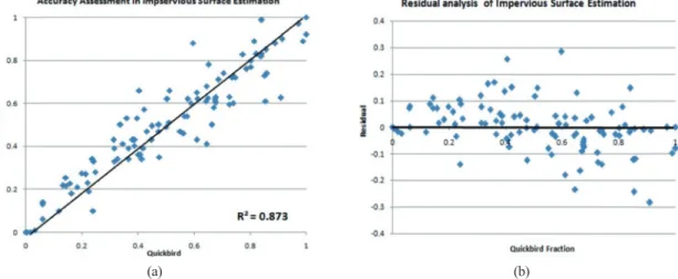
The QuickBird image used to test the accuracy of the classified results. As noted earlier, the QuickBird image acts as a convenient source for ground truth;

finer scaled to identify the spatial configuration of surface properties but because of high data volume the image covers only a small section of Phoenix. A simple ISODATA classification of the QuickBird image produced classes of impervious surfaces, vegetation, soil, and also water bodies. These are rescaled from 2.4 m to fit the 30 m of the Landsat TM pixels. Next, 100 pixels were randomly selected to measure accuracy by fitting a linear regression between spectral mixture fractions and referenced fractions from the QuickBird image. In an ideal case, the slope would be 1, the intercept 0, and the coefficient of determination (R

) at 1.0. The regression results in “y (spectral mixture) = 0.872x (QuickBird) + 0.066”, with a R

value of 0.873.

This is a very strong fit and demonstrates that the spectral mixture analysis produced reliable results. The relationship between modeled fractions estimated by spectral mixture analysis using Landsat TM and referenced fractions obtained from QuickBird image,

along with the residuals of the estimated impervious fractions are presented in Fig. 4a and 4b respectively.

Additionally, there are two types of error measurement to evaluate the accuracy of the fraction estimation. Root Mean Square (RMS) is the average absolute value of difference between modeled and measured fraction values for considering individual case. Bias means the difference between the modeled fractional value and reference fractional value of impervious surface (Powell et al., 2007). The RMS and bias for every image pixel are calculated to assess the performance of this model. The RMS model is assessed by the residual term e

or the RMS (3) (Wu and Murray 2003; Powell et al., 2007) over all bands (M):

RMS = ( e

/M) (3) Bias is the average of the error, and it indicates overall trends in overestimated or underestimated estimation (Powell et al., 2007):

bias = (Z

_ Z

)/ n (4) where Z

is the modeled fractional value of land-cover component k measured at pixel i, Z

is reference fractional value, and n is the number of samples (4) (Powell et al., 2007). Results present that the overall estimation RMS is 9.36%, and bias is 0.0017 for all

Σ

12

Σ

Fig. 4. (a) Accuracy Assessment of Impervious Surface Estimation Using Modeled Fractions from Landsat TM Sensor Image and Referenced Fractions obtained from the Finer Spatial Resolution QuickBird Sensor Image; (b) Residuals of the Estimated Impervious Fractions from QuickBird Sensor Image.

(a) (b)

samples. It means that this model presents well imperviousness information even if it tends to overestimate or underestimate.

4. Results

The results are based on the analysis is based on multiple regression models that explore the factors responsible for affecting the quality of stormwater runoff. It is premised by the assumption that imperviousness and vegetation cover, derived from remotely sensed data, are instrumental in determining the volume of runoff and the source of pollutant concentrations (Table 1).

The relationships between pollutant concentrations and land use types, total imperviousness, and vegetation cover can be expressed more statistically if multiple regression models are employed as the basis of the analysis. First, the individual relationships between

dependent variables and explanatory variables are explored using Pearson product moment coefficients, where the dependent variables are the pollutants; these are Biochemical Oxygen Demand (BOD

), Total Suspended Solids (TSS), Total Dissolved Solids (TDS), phosphorus (PHO), oil and grease (OIL), copper (Cu), zinc (Zn), and lead (Pb) (Table 2).

Independent or explanatory variables are maximum 5 minute Rainfall Intensity (RI), Population Density (PD), vegetation cover (NDVI), percentage of impervious surface (ISA), Drainage Area (DA), total stormwater runoff (cubic feet) (RO), number of dry days before rain (antecedent dry periods) (DD), percentage of commercial land use (LUC), percentage of industrial land use (LUI), percentage of undeveloped land use (LUN), and percentage of residential land use (LUR). The coefficients highlighted in bold in Table 2 indicate statistical significance at the 0.01 level. Of these, BOD

is highly positively correlated with industrial land use (0.546) but negatively correlated Table 1. Analysis to Identify Characterization of Stormwater Pollutants

Analysis

Data Characteristics Monitored data based on storm events Study Area Drainage basins of outfall monitoring sites

Method Constructing multiple regression models

Analysis & Interpretation Finding the decisive factors for stormwater quality

Table 2. Pearson Correlation Coefficients between Stormwater Pollutant Variables and Explanatory Variables at Storm Event Level

RI PD NDVI ISA DA RO DD LUC LUI LUN LUR

BOD

0.066 0.197 -0.535** 0.428* 0.010 0.497* 0.378 0.134 0.546** 0.046 0.052 TSS 0.241 0.425* -0.465* 0.133 0.307 0.074 0.602** 0.269 0.583** -0.212 -0.321 TDS 0.014 0.302 -0.093 0.405* 0.696** 0.273 0.482* 0.185 0.375 -0.268 -0.285 PHO 0.250 0.283 -0.563** 0.364 0.214 0.153 0.519** 0.145 0.556** -0.134 -0.043 OIL 0.032 0.219 0.380 0.299 0.142 0.255 0.409* 0.208 0.342 0.072 -0.276 Cu 0.148 0.339 -0.736** 0.475* 0.022 0.176 0.200 0.224 0.866** -0.151 -0.060 Zn 0.041 0.228 -0.609** 0.488** 0.083 0.179 0.495** 0.020 0.594** -0.232 -0.328 Pb 0.488** 0.028 0.519** 0.193 0.032 0.227 0.295 0.020 0.311 0.080 -0.314 Pollutants: BOD

=biochemical oxygen demand (mg/l); TDS = total dissolved solids (mg/l); TSS=total suspended solids (mg/l);

PHO=phosphorus (mg/l); OIL=oil and grease (mg/l); Cu=copper (ug/l); Zn=zinc (ug/l); Pb=lead (ug/l). Explanatory variables:

RO=total storm runoff (cubic feet); RI=maximum 5-minute rainfall intensity; LUR=percentage of residential land use;

LUI=percentage of Industrial land use; LUN=percentage of undeveloped land use; LUC=percentage of commercial land use;

DA=drainage area (Acres); PD=population density (per acre); NDVI=normalized difference vegetation index; ISA=percentage

of impervious surface area; DD=antecedent dry days; *correlation significant at the 0.05 level; **correlation significant at the

0.01 level.

with vegetation cover (-0.535). The significant variables that influence the amount of TDS are impervious surface (0.405), drainage area (0.696), and antecedent dry days (0.482). Moreover, TSS is highly correlated with dry weather days (0.602) and industrial land use (0.583). The amount of phosphorus is highly correlated to industrial land use (0.556), vegetation cover (-0.563), and dry weather periods (0.519). While heavy metals such as copper, zinc, and lead are closely related to industrial land use and vegetation cover.

Overall, the results seem to suggest that most stormwater pollutants are highly related to one type of urban land use, industrial.

Model building also includes the search for possible multicollinearity between the exploratory variables.

This is where two or more variables are highly correlated and loss of information may occur; the solution is to choose the one with the stronger significance level. Table 3 lists (in bold) possible multicollinearity between explanatory variables, such as NDVI with DA (correlation coefficient of 0.625, significant at the 0.01 level). After clearing for multicollinearity the independent variables used to explain stormwater quality are the percentage of industrial land use (LUI), total runoff (RO), antecedent dry days (DD), drainage basin area (DA), percentage of impervious surface (ISA), vegetation cover

(expressed by the NDVI), and rainfall intensity (RI).

These variables are used in eight separate multiple regression models; each focusing on one of the stormwater pollutants (Table 4). For instance, in model 1 biochemical oxygen demand (BOD

) is the response (or dependent) variable (Y) and both percentage industrial land use (LUI) (X1) and total runoff (RO) (X2) are the explanatory variables, expressed as BOD

= 20.53 + 0.54LUI + 3.34e _ 5RO. The value 20.53 is the constant (a), 0.54 and 3.34e-5 are the regression coefficients b

and b

for X

and X

respectively. And the model’s adjusted R

is significance at over 0.05 (SIG). Indeed all five models exceed the 0.05 levels and all five models produce low RMSE values (a measure of the differences between values predicted by the models and the observed values). All five models also test for non Bias_the probability of rejecting the null hypothesis of each model exceeded the significance level when the alternative was true and was less than or equal to the significance level when the null hypothesis is true.

In sum, the regression models reveal that most stormwater pollutants are strongly influenced by industrial land use as the most important surface variable. The heavy metals _ in particular, copper, lead and zinc _ are strongly affected by industrial land use, and more so than total impervious surface (ISA), which Table 3. Pearson Correlation Coefficients between Explanatory Variables

RI PD NDVI ISA DA RO DD LUC LUI LUN LUR

RI

PD .3

NDVI .114 -.119

ISA .172 .535** -.177

DA -.054 -.327 .625** -.195

RO -.047 -.19 .034 -.233 .533**

DD .211 -.057 -.012 .029 .059 -.113

LUC .271 .787** -.144 .498** -.34 -.172 -.043

LUI -.176 .29 .1 .406* .334 -.008 .052 -.367*

LUN .194 -.202 -.152 -.331 -.370* -.28 -.04 -.284 -.23

LUR -.085 .064 -.129 .464** -.22 .121 -.002 .074 -.807** -.138

See Table 2 for variable descriptions

is only significant in explaining total dissolved solids (TDS). For example, the drainage basins of SR30 is mainly used for industrial, agricultural, residential, and commercial land use areas. Industrial land use of industrial parks, metal management plants, steel companies and factories can affect the location of stormwater monitoring sites and the amounts of stormwater pollutants (Fig. 5). The drainage area of SR49 mainly consists of industrial (29.22%) and agricultural (34.31%) land use. There are many industrial companies, agricultural areas, cow milk farms, and transportation and warehouse centers (Fig.

6). Indeed, runoff (RO) which initially was speculated as an important factor_and a direct result of impervious surfaces_is only evident in model 1. However, the climatic variables, dry days (DD) and maximum rainfall intensity (RI) are evident in all the models, but can be almost considered as constants given the relatively small geographic area of Phoenix. Lastly, vegetation cover (expressed as an NDVI value) appears significant in models 4 to 8. Their coefficients are as expected negative and support the assumption that green areas absorb runoff and thereby reduce the transport of waterborne pollutants.

Fig. 5. (a) SR30 monitoring site and main land use in basin and (b) land uses and facilities of SR30 basin (Data: QuickBird and taken by author’s fieldwork).

Table 4. Multiple Regression Models to Explain Factors of Stormwater Quality

Model R R2 (ADJ) Regression Model SIG RMSE Bias

1 0.769 0.592 (.551) BOD

= 20.53 + 0.54LUI + 3.34E-5RO 0.00 0.77 0.00

2 0.774 0.599 (.566) TSS = 52.28 + 4.71LUI + 5.03DD 0.00 0.76 0.00

3 0.854 0.729 (.692) TDS = _157.98 + 3.29ISA + 0.09DA + 4.31DD 0.00 0.71 0.00 4 0.743 0.552 (.491) PHO = 0.63 + 0.01LUI _ 1.50NDVI + 0.01DD 0.00 0.72 0.00 5 0.531 0.282 (.215) OIL = 6.37 + 0.02LUI _ 12.02NDVI + 0.06DD 0.02 0.71 0.00

6 0.896 0.803 (.787) Cu = 75.94 + 1.71LUI _ 262.10NDVI 0.00 0.69 0.00

7 0.750 0.563 (.508) Zn = 292.29 + 3.39LUI _ 988.62NDVI + 3.40DD 0.00 0.67 0.00 8 0.670 0.449 (.380) Pb = 29.61 + 0.30LUI _ 112.42NDVI + 16.42RI 0.00 0.65 0.00 See Table 2 for variable descriptions

SIG=significance at the 0.05 level; ADJ=adjusted R

square; RMSE=root mean square error; Bias=the average of residual errors

(a) (b)

5. Conclusion and Discussion

The problem of flash flooding and heavy runoff is particularly acute in cities built in arid climatic zones.

Here storms are frequently intense and cause loose sediment and pollutants to be washed across sun- hardened surfaces into hydrological basins causing widespread degradation of water quality. The main factors that typically dictate the volume of runoff and hence affect the quality of the water across a city are topographic; in particular land use and land cover.

Remote sensing is a technology that facilitates the rapid and widespread collection of digital data that represent the two most influential urban land cover types;

imperviousness and biophysical areas (vegetation and soil). In addition, the wealth of digital data collected by satellite remote sensing allows continuous measurements of imperviousness and vegetation percentages using two statistical models, spectral mixture analysis and the NDVI respectively. These two techniques were demonstrated using a remotely sensed image from the Landsat TM sensor representing the arid city of Phoenix. Landsat TM images have a long

history, are readily accessible, and cover entire urban areas. They are ideal vehicles for frequent and consistent surveillance, capable of measuring precise expansions of imperviousness and proportions of green space.

The main assumption is that imperviousness, vegetation cover and land use would be responsible for the spatial distribution of stormwater pollutants. To support this, multiple regression models for each of the eight solid-suspended and heavy metal pollutants were built from 30 storm events at seven outflow monitoring sites. The results indicated that stormwater pollutants are highly concentrated on industrial and commercial land uses. Conversely, basins characterized by smaller patches of industrial land use and a high ratio of undeveloped land, contained the least amounts of pollutants. These general findings were supported by the results from the multiple regression models, where stormwater quality again deteriorated when associated with industrial land use and indeed general impervious surfaces. Each of the pollutants, whether water suspended solids or heavy metals, had positive relationships with impervious surfaces and/or industrial Fig. 6. (a) SR49 monitoring site and main land use in basin and (b) land uses and facilities of SR49 basin (Data: QuickBird and taken

by author’s fieldwork).

(a) (b)

land use. And as anticipated, each had negative relationships with vegetation cover. Not surprisingly, residential land use is somewhere between and did not play an active role in influencing levels of stormwater pollutant loads.

Admittedly, these findings are not unexpected. What was achieved was the development of a spatial- statistical methodology that takes advantage of the data collection convenience of satellite sensor imagery, beyond the sparsity of conventional point-based sampling, for identifying evidence for rapid consequences of urbanization. Indeed, this raises the question of spatial dependence in the results given that the analyses were conducted from water quality data from seven outfall locations. Although difficult to control all spatial autoregressive relationships, these locations were spread across the whole of Phoenix and were adjacent to all the different types of land uses.

Also, there are several limitations of our work and suggestion for future studies. Above all, sub-pixel classification approaches have the limitation in assessing of the accuracy assessment compared to per- pixel and object-based classification. Future research is required to select area-based samples through ground- truth survey, instead of high spatial resolution imagery, for more accurate accuracy assessment. Additionally, key urban sources of heavy metal include building roofs, pavements, road dusts, agricultural support industries, chemical and associated produce manufacturing, commercial livestock processing industries, metal product manufacturing, meter processing manufacturing, motor vehicle service facilities, and catchment soil quality, etc (Davis et al., 2001; Kennedy and Sutherland, 2008; Wicke et al., 2012). Therefore, stormwater quality models, especially, soil quality, dry and wet deposition, atmospheric emission, and other factors as well as urban land use and land cover influenced on the concentrations of heavy metals of Cu, Pb, and Zn.

Future research should target these to advance the

mechanistic understanding of each heavy metals factor contributions.

Lastly, the work supports current debates on urban public policies that advocate environmental sustainability and the more recent focus on urban livability. Both have quality of life as their central objective and both develop plans that harmonize construction with nature and the optimal balance between low environmental pollution and need for economic and commercial progress. Indeed, the balance with nature frequently spawns analogies with ecology. For example, the urban carrying capacity predicates the notion of a viable ecological limit to urban population, and metabolism models endeavor to strike equilibrium between urban input resources and output waste. Excessive urban runoff can be considered as waste, particularly when solids and heavy metals are washed across the city. Planners should be aware of these hazards and should attempt to approve new construction and propose redevelopment that both steer away from vast unbroken impervious surfaces, and instead advocate more fragmented landscapes that harmonize built and biophysical spaces with respect to efficient transport networks and access to public and commercial facilities.

References

Adams, J.B. and F. Papa, 2000. Urban Stormwater Management Planning with Analytical Probabilistic Models, Wiley, New York, USA, ISBN-13: 978-0471332176.

Arnold, C.L. and C.J. Gibbons, 1996. Impervious Surface Coverage: The Emergence of a Key Environmental Indicator, Journal of the American Planning Association, 62: 243-258.

Bailang, Y., H. Liu, J. Wu, Y. Hu, and L. Zhang, 2010.

Automated derivation of urban building density

information using airborne LiDAR data and

object based method, Landscape and Urban Planning, 98: 210-219.

Brabec E., S. Shulte, and P.L Richards, 2002.

Impervious Surfaces and Water Quality: A Review of Current Literature and its Implications for Watershed Planning, Journal of Planning Literature, 16: 499-514.

Brattebo, B.O. and D.B. Booth, 2003. Long-term Stormwater Quantity and Quality Performance of Permeable Pavement Systems, Water Resources, 37: 4369-4376.

Brezonik, P.L. and T.H. Stadelmann, 2002. Analysis and Predictive Models of Stormwater Runoff Volumes, Loads, and Pollutant Concentrations from Watersheds in the Twin Cities Metropolitan Area, Minnesota, USA, Water Resources, 36: 1743-1757.

Bultler, D., and J.W. Davies, 2011. Stormwater management. In D. Butler and W. Davies (Eds), Urban Drainage (pp.519-550), CRC Press, Boca Raton.

Canters, F., O. Batelaan, T.V. Voorde, J. Cjormanski, and B. Verbeiren, 2011. Use of impervious surface data from remote sensing in distributed hydrological modeling of urban areas. In X.

Yang (Ed.), Urban Remote Sensing: Monitoring, Synthesis and Modeling in the Urban Environment (pp. 255-273), Wiley, Chichester.

Carlson, T.N, 2004. Analysis and Prediction of Surface Runoff in an Urbanizing Watershed Using Satellite Imagery, Journal of the American Water Resources Association, 40: 1087-1098.

Carlson, T.N., 2008. Impervious Surface Area and its Effect on Water Abundance and Water Quality.

In Q. Weng (Ed.), Remote Sensing of Impervious Surface(pp. 353-367), Taylor & Francis, Boca Raton.

Carter, T. and C.R. Jackson, 2007. Vegetated Roofs for Stormwater Management at Multiple Spatial Scales, Landscape and Urban Planning, 80:

84-94.

City of Phoenix, Arizona, 2003 to 2008. Municipal Separate Storm Sewer System: Annual Report for the Year Ending June 30, 2003 to June 30, 2008, NPDES permit NumberAZS000003.

Conway, T.M, 2007. Impervious surface as an indicator of pH and specific conductance in the urbanizing coastal zone of New Jersey, USA, Journal of Environmental Management, 85(2):

308-316.

Coroza, O., D. Evans, and I. Bishop, 1997. Enhancing Runoff Modeling with GIS, Landscape and Urban Planning, 38: 13-23.

Cruise, J.F., C.A. Laymon, and O.Z. Al-Hamdan, 2010.

Impact of 20 years of Land-cover Change on the Hydrology of Streams in the Southeastern United States, Journal of the American Water Resources Association, 46(6): 1159-1170.

Davis, A.P., M. Shokouhian, and S. Ni, 2001. Loading estimates of lead, copper, cadmium, and zinc in urban runoff from specific sources, Chemosphere, 44: 997-1009.

Dougherty, M., R.L. Dymond, S.J. Goetz, C.A. Jantz, and N. Goulet, 2004. Evaluation of Impervious Surface Estimates in a Rapidly Urbanizing Watershed, Photogrammetric Engineering &

Remote Sensing, 70: 1275-1284.

Ganbaatar, G. and K.S. Lee, 2013. Classification of crop lands over Northern Mongolia using multi-temporal Landsat TM data, Korean Journal of Remote Sensing, 29 (6): 611-619.

Gnecco, I., C. Berretta, L.G. Lanza, and P. La Barbera, 2005. Storm-water Pollution in the Urban Environment of Genoa, Italy, Atmospheric Research, 77: 60-73.

Gobel, P., C. Dierkes, and W.G. Coldewey, 2007.

Stormwater runoff concentration matrix for urban areas, Journal of Contaminant Hydrology, 91(1-2): 26-42.

Goetz, S.J., K.W. Robb, J.S. Andrew, Z. Elizabeth,

and S. Erika, 2003. IKONOS Imagery for Resource Management: Tree cover, Impervious Surfaces, and Riparian Buffer Analyses in the Mid-Atlantic Region, Remote Sensing of Environment, 88: 195-208 Jat, M.K., D. Khare, P.K. Garg, and V. Shankar, 2009.

Remote Sensing and GIS-based Assessment of Urbanization and Degradation of Watershed Health, Urban Watershed Journal, 6: 251-263.

Jiang, Z., A.R. Huete, J. Chen, Y. Chen, J. Li, G. Yan, and X. Zhang, 2006. Analysis of NDVI and Scaled Difference Vegetation Index Retrievals of Vegetation Fraction, Remote Sensing of Environment, 101: 366-378.

Jung, M. and E. Chang, 2013. Land-cover vegetation change detection based on harmonic analysis of MODIS NDVI time series data, Korean Journal of Remote Sensing, 29 (4): 351-360.

Kennedy, P. and S. Sutherland, 2008. Urban Sources of Copper, Lead and Zinc, Auckland Regional Council, Takapuna, New Zealand.

Kim, J.P., K.W. Park, W. Jung, K.S. Han, and G. Kim, 2013. Application of high resolution multi- satellite precipitation products and a distributed hydrological modeling for daily runoff simulation, Korean Journal of Remote Sensing, 29 (2): 263-274 (in Korean with English abstract).

Lee, J.G. and J.P. Heaney, 2003. Estimation of Urban Imperviousness and its Impacts on Storm Water Systems, Journal of Water Resources Planning and Management, 129: 419-426.

Leprieur, C., Y.H. Kerr, S. Mastorchio, and J.C.

Meunier, 2000. Monitoring Vegetation Cover across Semi-arid Regions: Comparison of Remote Observations from Various Scales, International Journal of Remote Sensing, 21:

281-300.

Liu, H. and L. Wang, 2008. Mapping Detention Basins and Deriving their Spatial Attributes from

LiDAR Data for Hydrological Applications, Hydrological Processes, 22: 2358-2369.

Liu, X., X. Li, Y. Chen, Z. Tan, S. Li, and B. Ai, 2010.

A New Landscape Index for Quantifying Urban Expansion Using Multi-temporal Remotely Sensed Data, Landscape Ecology, 25: 671-682.

Lopes, T.J., K.D. Fossum, J.V. Phillips, and J. Monical, 1994. Statistical Summary of Selected Physical, Chemical, and Microbial Characteristics and Estimated of Constituent Loads in Urban Stormwater, USGS Water Resources investigations Report 94-4240 (USGS, Maricopa County, AZ).

Martin, P.H., E.J. LeBoeuf, and J.P. Dobbins, 2005.

Interfacing GIS with Water Resource Models:

A State-of-the-Art Review, Journal of the American Water Resources Association, 41(6):

1471-1487.

Matthies, M., J. Berlekamp, S. Lautenbach, N. Graf, and S. Reimer, 2006. System Analysis of Water Quality Management for the Elbe River Basin, Environmental Modeling Software, 21:

1309-1318.

Morgan, K.M., L.W. Newland, E. Weber, and A.B.

Busbey, 1993. Using SPOT Satellite Data to Map Impervious Cover for Urban Runoff Predictions, Toxicological Environmental Chemistry, 40: 11-16.

Myint, S.W. and G.S. Okin, 2009. Modelling Land- Cover Types Using Multiple Endmember Spectral Mixture Analysis in a Desert City, International Journal of Remote Sensing, 30:

2237- 2257.

Newman, P.W.G., 1999. Sustainability and Cities:

Extending the Metabolism Model, Landscape and Urban Planning, 44: 219-226.

Nouh, M. and N. Al-Noman, 2009. Regression Models

for the Prediction of Water Quality in the

Stormwater of Urban Arid Catchments,

Canadian Journal of Civil Engineering, 36:

331-344.

Pitt, R., and S.E. Clark, 2008. Integrated Stormwater Management for Watershed Sustainability, Journal of Irrigation and Drainage Engineering, 134 (5): 548-566.

Powell, R. L., D. A. Roberts, P. E. Dennison, and L. L.

Hess, 2007. Sub-pixel mapping of urban land cover using multiple endmember spectral mixture analysis: Manaus, Brazil, Remote Sensing of Environment, 106: 253-267.

Schiff, R., and G. Benoit, 2007. Effects of impervious cover at multiple spatial scales on coastal watershed streams, Journal of the American Water Resources Association, 43(3): 712-730.

Shao, G. and J. Wu, 2008. On the Accuracy of Landscape Pattern Analysis Using Remote Sensing Data, Landscape Ecology, 23: 505- 511.

Shin, D.H., Y.M. Noh, S.K. Shin, and Y.J. Kim, 2014.

Development of lidar detection system for improvement of measurement range (Combined photon counting detection and analog-to-digital signal), Korean Journal of Remote Sensing, 30 (2): 251-258.

Simon, J.A., J.W. Snodgrass, R.E. Casey, and D.W.

Sparling, 2009. Spatial correlates of amphibian use of constructed wetland in an urban landscape, Landscape Ecology, 24: 361-373.

Slavin, M.I, 2011. The rise of the urban sustainability movement in America. In M.I. Slavin (Ed.), Sustainability in America’s Cities (pp.1-19), Island press, Washington.

Song, A., Y. Han, Y. Kim, and Y. Kim, 2014. Spectral mixture analysis using modified IEA Algorithm for forest classification. Korean Journal of Remote Sensing, 30 (2): 219-226 (in Korean with English abstract).

Stone, B. and J.L. Bullen, 2006. Urban Form and Watershed Management: How Zoning

Influences Residential Stormwater Volumes, Environment and Planning B, 33: 21-37.

Thanapura, P., D.L. Helder, S. Burkhard, E. Warmath, M. O’Neill, and D. Galster, 2007. Mapping Urban Land Cover using QuickBird NDVI and GIS Spatial Modeling for Runoff Coefficient Determination, Photogrammetric Engineering and Remote Sensing, 73: 57-65.

Thurston, H.W., H.C. Goddard, D. Szlag, and B.

Lemberg, 2003. Controlling Storm-water Runoff with Tradable Allowances for Impervious Surfaces, Journal of Water Resources Planning and Management, 129:

409-418.

Tong, S.T.Y. and W. Chen, 2002. Modeling the Relationship between Land Use and Surface Water Quality, Journal of Environmental Management, 66: 377-393.

US Census Bureau, 2010. [http: //www.census.gov/].

USEPA, 2000. Storm Water Phase II Compliance Assistance Guide, EPA 833-R-00-002 Office of Water, Washington, DC.

USEPA, 2003. Protecting Water Quality from Urban Runoff, EPA 841-F-03-003 Office of Water, Washington, DC.

Van Kamp, I., K. Leidelmeijer, G. Marsman, and A.

de Hollander, 2003. Urban Environmental Quality and Human Well-being: Towards a Conceptual Framework and Demarcation of Concepts; a Literature Study, Landscape and Urban Planning, 65: 5-18.

Wedding, G.C. and D. Crawford-Brown, 2007.

Measuring Site-level Success in Brownfield Redevelopments: A Focus on Sustainability and Green Building, Journal of Environmental Management, 85: 483-495.

Weng, Q, 2010. Remote sensing and GIS integration:

Theories, Methods, and Applications, McGrewHill, New York.

Weng, Q, 2012. Remote sensing of impervious surfaces

in the urban areas: requirements, methods, and trends, Remote Sensing of Environment, 117:

34-49.

Wicke, D., T.A. Cochrane, and A. O’Sullivan, 2012.

Build-up dynamics of heavy metals deposited on impermeable urban surfaces, Journal of Environmental Management, 113: 347-354.

Wu, C.S. and A.T. Murray, 2003. Estimating Impervious Surface Distribution by Spectral Mixture Analysis, Remote Sensing of

Environment, 84: 493-505.

Wu, J., G.D. Jenerette, A. Buyantuyev, and C.L.

Redman, 2011. Quantifying spatiotemporal patterns of urbanization: The case of the two fastest growing metropolitan regions in the United States, Ecological Complexity, 8(1): 1-8.

Xiao, F., M.F. Simcik, and J.S. Gulliver, 2012.

Perfluoroalkyl acids in urban stormwater

runoff: Influence of land use, Water Research,

46: 6601-6608.