A Microscopic Analysis on the Fundamental Diagram and Driver Behavior
교통기본도와 운전자 행태에 대한 미시적 분석
Kim, Taewan 김`태`완 Membership·Associate Professor, Department of Urban Engineering Chung-Ang University (E-mail:[email protected])
ABSTRACT
PURPOSES :The fundamental diagram provides basic information necessary in the analysis of traffic flow and highway operation. When traffic flow is congested, the density-flow points in the fundamental diagram are widely scattered and move in a stochastic manner. This paper investigates the pattern of density-flow point transitions and identifies car-following behaviors underlying the density-flow transitions. . METHODS :From a microscopic analysis of 722 fundamental diagrams of NGSIM data, a total of 20 transition patterns of fundamental diagrams are identified. Prominent features of the transition patterns are explained by the behavior of the leader and follower.
RESULTS :It is found out that the average speed and the speed difference between the leader and the follower critically determine the density-flow transition pattern. The density-flow path is very sensitive to the values of vehicle speed and spacing especially at low speed and high density such that most fluctuations in the fundamental diagram in the congested regime is due to the noise of speed and spacing variations.
CONCLUSIONS :The result of this study suggests that the average speed, the speed difference between the leader and the follower, and the random variations of speed and spacing are dominant factors that explain the transition patterns of a fundamental diagram.
Keywords
fundamental diagram, driver behavior, traffic hysteresis, congested traffic, NG-SIM data
1. INTRODUCTION
Car-following models, which describe the rule by which a vehicle follows its leader, have become the most important topic in traffic engineering. Even though car-following models have been developed since 1950s, many phenomena occurring in traffic stream have not been sufficiently explained, especially in congested traffic. The most well- known car-following model would be the GHR (Gazis- Herman-Rothery) model (Chandler et al., 1958; Gazis et al.,
1959; Edie, 1961; Gazis et al., 1961). According to the car following model, a vehicle’s acceleration rate is influenced by its speed, speed difference, and spacing with the vehicle in front. Numerous researchers have paid attention to determining the values of parameters in the GHR model (Brackstone and Mac Donald, 1999). It is known that, for specific values of parameters, the GHR model can reproduce the most prominent traffic stream models, such as the Greenshields model and the Greenberg model (Greenshields, Main Author : Kim, Taewan, Associate Professor
Department of Urban Engineering, Chung-Ang University, 84 Heuksuk-ro, Dongjak-gu, Seoul, 156-756, Korea Tel : +82.2.820.5846 Fax : +82.2.825.4709 email : [email protected]
International Journal of Highway Engineering http://www.ksre.or.kr/
ISSN 1738-7159 (Print) ISSN 2287-3678 (Online)
International J. Highw. Engineering Vol. 14 No. 6 : 183-190 December 2012 http://dx.doi.org/10.7855/IJHE.2012.14.6.183
1934; Greenberg, 1959). Another approach to car-following models is based on the safety distance or collision avoidance rule. This approach presumes that drivers control their speeds in order to maintain a safe distance and avoid collision with the leading car. The car-following equations of these models contain vehicle speed and spacing terms, which also can be easily transformed to the traffic stream models (Pipes, 1953;
Koemtani and Sasaki, 1958; Gipps, 1981; Zhang and Kim, 2005). Other approaches to car following model include linear model, psycho-physiological model, and cellular automata model (Helly, 1959; Leutzbach and Wiedemann, 1986; Nagel, 1996; Nagel and Schreckenberg, 1996).
However, car following models mentioned above rely on a single or several car-following equations and cannot thoroughly explain driver behavior in complicated traffic conditions.
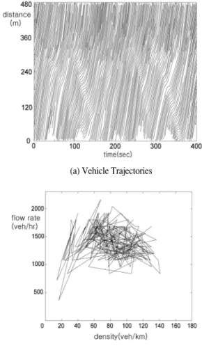
Fig. 1 shows the vehicle trajectory and fundamental diagram of Interstate-405 in the vicinity of LA, California, drawn from the aerial data collected in 1985 (FHWA, 1985).
In Fig.1 (a), we can see that the traffic is congested and vehicles are experiencing stop-and-go traffic. Fig. 1 (b) is the
fundamental diagram drawn from the same data, in which we can find that the observation points of density-flow are widely scattered and move in a stochastic manner. The widely scattered region of flow-density observations may be partly explained by the diversity of drivers and vehicle characteristics, lane changing, and traffic hysteresis.
A number of empirical studies investigated the features of fundamental diagram suggesting single regime type (6-7), dual regime type (Hillegas et al., 1974; Hall et al., 1991), reversed lambda (Koshi et al, 1984) or inverted V type (Newell, 1993). However, these traffic stream models represent the aggregate (or average) relation of density-flow and fall short in explaining the complicated transition of flow-density observation points as in Fig.1(b).
The scattering of flow-density points has been reported by a number of papers (Kerner and Rehborn, 1996; Kerner, 1998; Yeo and Skarbadonis, 2009). The factors that partly contribute to the scattering of flow-density are claimed to be drivers’over reactions and late responses, lane changes (Laval, 2005; Chiabaut et al., 2009) and traffic hysteresis (Newell, 1965; Treiterer and Myers, 1974; Zhang, 1999;
Laval, 2010).
The fundamental diagram represented by density-flow plot contains significant information on the congested traffic, such as drivers’behavioral characteristics, traffic hysteresis, and wave speed. However, sufficient explanations are not provided regarding the stochastic features of density-flow points transitions. The purpose of this paper is to investigate and identify driver behaviors that are not discussed in the previous car-following models through the analysis of transition patterns of density-flow points in the fundamental diagram
2. TRANSITION PATTERN ANALYSIS
The fundamental diagram can be obtained from detector data or vehicle trajectory data. Because detector data aggregate vehicle count or speed for a specified time period, averaging effects exist in the detector data. In order to investigate the specific influence of driver behavior on the fundamental diagram, detector data, which have averaging effects, are not appropriate. In this paper, NGSIM data (FHWA, 2006), which provide vehicle trajectories for a Fig. 1 Vehicle Trajectory and Fundamental Diagram of I-405
(a) Vehicle Trajectories
(b) Fundamental Diagram
congested traffic, is used for the microscopic analysis of fundamental diagram. Among the NGSIM data, the I-80 data set in the time interval of 5:00~5:15 is selected for the analysis because the traffic in the data is moderately congested and scattering of flow-density points can be explicitly obtained from the data. The density and flow rate are estimated for every pair of vehicle to eliminate aggregation error and the vehicles that have changed travel lanes are excluded from the analysis. From the data, a total of 722 pairs of vehicle trajectories are identified and corresponding fundamental diagrams are plotted. The flow and density are estimated following Edie’s generalized definition of traffic variables (Laval, 2010). When we have n vehicles inside an arbitrary region A in a time-space diagram, the density ( ) and flow rate ( ) is estimated by
where, and represent the vehicle’s travel time and distance inside the region A, respectively, and represents the area of the region A. As is shown in Fig.2, the arbitrary region A is constructed as a parallelogram containing a pair of vehicles.
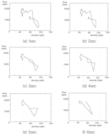
The selection of measuring time step ( ) is essential for the proper estimation of flow rate and density. If the time step is too short, trivial variations of flow rate and density can be captured in the fundamental diagram, which may interrupt identifying distinctive features of fundamental diagram. On the other hand, if the time step is too long, averaging effects may be produced. In Fig.3, fundamental diagrams for different time steps are plotted for a pair of vehicles (vehicle
ID 1690 and 1696). We can see that trivial variations of flow rate and density are captured when the time step is 1sec or 2sec and averaging effects are produced when the time step is 5sec or 6sec. Therefore, a time step of 3sec is taken for the analysis of 722 pairs of vehicle trajectories. Fig. 4 depicts two examples from the 722 density-flow plots. If the pair of vehicles travels the stretch of the freeway with relatively high speed, the number of observation points is relatively small and density-flow path shows a simple line. On the contrary, if the traffic is congested and the pair of vehicles travels the stretch of the freeway with lower speed, the number of observation points would be larger and density-flow paths will be more complicated.
The empty circles in the figure represent the starting points of density-flow point transition paths and the filled circles (1)
(2)
Fig. 2 Estimation of Flow Rate and Density for a Pair of Vehicles
Fig. 3 Fundamental Diagrams Drawn for Different Time Steps
Fig. 4 Simple Transition and Returning Paths
(a) 1sec (b) 2sec
(c) 3sec (d) 4sec
(e) 5sec (f) 6sec
(a) (b)
represent the ending points of the paths. In Fig. 4 (a), the density-flow path shifts to the left side of the starting point and does not return to the starting point. On the other hand, in Fig. 4 (b), we can see a closed curved line, in which the density-flow path returns to the point that it previously passed.
In fact, the returning path in Fig. 4 (b) can be divided into two paths of shifted line and, if observation time was long enough, the path in Fig. 4 (a) may return to the initial point.
Our concern in this research is not in the whole picture of flow-density path for a long time period but in the snapshot of the path and for simplicity our investigation will mainly deal with the factors that can characterize the patterns of density- flow point shifting.
The first factor that can characterize the transition of density-flow path is whether the speed or density has changed during the transition. Speed and density (or spacing) are important parameters of car-following models and can describe driver’s behaviors explicitly. On the contrary, flow rate is not directly related to an individual vehicle’s behavior.
In Fig. 5 (a), except several points around the ending point, the path moves linearly and the speed does not change during the transition. If both the leader and follower of the pair of vehicle do not change their speeds, the density also should be constant. Therefore, for the case of Fig. 5 (a), when we say
‘constant speed’, the speed is constant for an average value but for the individual vehicle of leader and follower, their speeds may change. In Fig. 5 (b), the density does not change while the speed increases during the transition. This is only possible when two vehicles simultaneously and identically change their speeds. In Fig. 5 (c), both the speed and density change during the transition. A horizontal path of constant flow rate may exist. However, the speed and density also changes for the constant flow rate and because the flow rate is not significant in the perspective of driver behavior, we do not define an exclusive pattern for the constant flow rate.
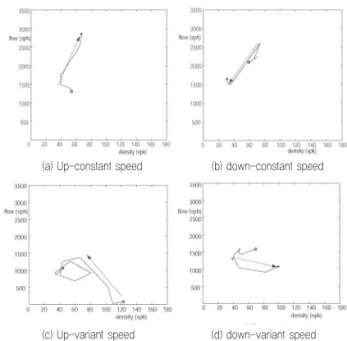
The second factor deals with the direction of the transition.
In the case that the speed is constant, if the path of flow- density moves upward, the flow/density increases (Fig. 6 (a)), and if the path of flow-density moves downward, the flow/density decreases (Fig. 6 (b)). For the other cases such as Fig. 5 (b) and Fig. 5 (c), we define ‘upward’as the path moving in the direction that speed increases and ‘downward’
as the path moving in the direction that the speed decreases.
The density can increase or decrease for both cases of upward and downward because in this pattern analysis we do not necessarily presume decreasing function of density-flow.
The third factor deals with whether the path is linear (Fig. 7 (a)), clockwise curved (Fig. 7 (b)) or counter clockwise curved (Fig. 7 (c)). A precise quantitative classification between ‘linear’and ‘curve’is not developed in this paper, but a visual determination is applied ad hoc.
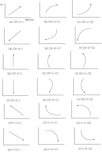
In summary, we can categorize the pattern of flow-density transition with three factors as seen in Fig. 8. With the combination of these three factors, theoretically we can have 18 different patterns (3×2×3=18) of flow-density Fig. 5 Constancy (Factor 1): Constant Speed,
Constant Density, Variant Speed and Density
Fig. 6 Direction (Factor 2): Up and Down
Fig. 7 Curvature (Factor 3): Linear, Clockwise, and Counter clockwise
(a) Constant speed (b) Constant density (c) Variant speed and denstiy
(a) Up-constant speed (b) down-constant speed
(c) Up-variant speed (d) down-variant speed
(a) Linear (b) Clockwise (c) Counter-clockwise
transitions. Here, for the first factor, the terms ‘CS’, ‘CD’, and ‘V’represent constant speed, constant density, and variant speed and density, respectively. For the second factor,
‘U’represents upward and ‘D’represents downward. For the third term, ‘L’, ‘C1’, and ‘C2’represent linear, clockwise, and counterclockwise, respectively.
Exceptions of the 18 patterns include the zigzag pattern and concentration pattern. Zigzag pattern refers to a path moving in such an irregular and stochastic manner that none of the 18 patterns can be applicable (Fig. 9 (a)). If we consider that the measurement time step is only 3sec and vehicles cannot change their flow, speed and density in such a short time, it is difficult to explain the zigzag pattern with existing car-following theories. However, further investigation has shown that the zigzag pattern is a result of small and trivial disturbances of speed and density. A detailed explanation will be in the following section. The second exception, the concentration pattern refers to a path in which variations of density and flow are so small and the path remains in a small area. Fig. 10 depicts empirical density-flow paths that correspond to the theoretically presumed 18 patterns of transition as in Fig. 9.
Some plots have additional observation paths before the starting points or after the ending points. However, for a clear comparison with Fig. 8, unimportant sections of the path outside of the starting points and the ending points were deliberately omitted. In Fig. 10, the empirical transition patterns generally coincides with theoretically derived patterns.
Considering those 18 patterns are all the possible shifting patterns in a 2-dimensional domain, if we identify the car- following behaviors that correspond to the 18 patterns, we may understand all possible car-following behaviors in a real traffic flow.
Fig. 8 Patterns of Density-Flow Transition
Fig. 9 Zigzag and Concentration Patterns
Fig. 10 Empirical 18 Patterns Corresponding to the Theoretical Patterns
(a) zig-zag (b) concentration
3. DRIVER BEHAVIOR ANALYSIS
In this section, we will identify the car-following behaviors underlying the 18 patterns in Fig. 10 by plotting the speed profiles of the following and leading vehicles.
However, plotting speed profiles for all the patterns in Fig.
10 would be unnecessary and we will plot several representative patterns. Fig. 11 depicts the speed profiles for the patterns in Fig. 10 (d) and (e). Here the speed is the average speed of the measurement time step, 3seconds. The solid line represents the speed of the leading vehicle and the dotted line represents the speed of the following vehicle. The thick solid line represents the average (arithmetic) value of the speeds of the leading and following vehicles. As is seen in Fig. 11 (a), the speed of the leader increases and then decreases. In contrast, the speed of the follower decreases and then increases. By chance, the average speed of these two vehicles becomes almost constant, explaining how the pattern ‘CS’is made. In Fig. 11 (a), the speed of the leader is faster than the speed of the follower. This speed difference reduces the spacing and transition path moves downward. If the speed of the leader is slower than the speed of the follower, the transition path would move upward. Other speed profiles that can produce the same pattern of ‘CS-D- L’may exist, but listing all the speed profiles corresponding to ‘CS-D-L’would be a burden and unnecessary at this time.
Fig.11 (b) corresponds to Fig. 10 (e). Initially, the vehicles decelerate and then accelerate. At the time of 30sec (10×
3sec), the speed recovers to the speed at the time of 18sec.
Because the speed profile is concaved and the speed of the leader is higher than the speed of the follower, the density- flow path is ‘D-C1’. If the speed profile is concaved and the speed of the leader is lower than the speed of the follower, the density-flow path is ‘U-C2’.
Fig. 12 depicts the speed profiles for the patterns in Fig. 10 (j) and (h). As is seen in Fig. 12 (a), the leader and follower reduce their speeds simultaneously and the speed differences
are negligible. This explains why the density is constant while the average speed decreases in Fig. 10 (j).
In Fig. 12, both the leader and follower increase their speeds. Before 12sec, the speed of the leader is higher than the speed of the follower. However, after 12sec, the speed of the follower is higher than the speed of the leader.
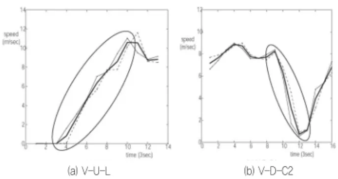
Accordingly, we can see that the path in Fig. 12 (h) initially moves upward left-slanted and then moves upward right- slanted. Fig. 13 (a) depicts the speed profiles of the pattern in Fig. 10 (m). As is seen, both the speeds of the leader and follower increases and the speed of the leader is consistently higher than the speed of the follower. This explains the path in Fig. 10 (m) moves upward to the left. Fig. 13 (b) depicts the speed profiles of the pattern in Fig. 10 (r). The average speed consistently decreases and the speed difference between the leader and the follower gradually increases during the time of 27~33sec. This explains the path in Fig. 10 (r) moves downward and counter-clockwise.
In Fig. 14 (a), the speeds of the leader and the follower are very low, mostly under 4m/sec, and frequently changes. The speed differences between the leader and follower are negligible. However, corresponding path in Fig. 9 (a) shows very complicated movement. In contrast, the speed differences between the leader and follower in Fig. 14 (b) is relatively large while corresponding path in Fig. 9 (b) stays in a small area. Comparing Fig. 14 (a) and (b), we can see that Fig. 11 Speed Profiles for Constant Speed
Fig. 12 Speed Profiles for Constant Density
Fig. 13 Speed Profiles for Variant Speed and Density
(a) CS-D-L (b) CS-D-C1
(a) CS-D-L (b) CS-U-C1
(a) V-U-L (b) V-D-C2
at low speed and high density, the density-flow path is very sensitive to the values of vehicle speed and spacing. In contrast, at high speed and low density, the density-flow path is stolid to the values of vehicle speed and spacing.
4. CONCLUSIONS
The fundamental diagram, representing the relations of density and flow rate, is very important for the analysis of traffic flow. When traffic flow is congested, the observation points of density-flow are widely scattered and move in a stochastic manner. This paper investigates the pattern of density-flow point transitions and identifies car-following behaviors underlying the density-flow transitions. From a microscopic analysis of 722 fundamental diagrams of NGSIM data, it is found that 3 factors dominate in defining the transition patterns. They are constancy of speed and density, movement direction, and curvedness. A total of 20 patterns are theoretically presumed through the combination of the three factors and the existence of the patterns is empirically confirmed. It is also found out that the average speed and the speed difference between the leader and the follower critically determine the density-flow transition pattern. The density-flow path is very sensitive to the values of vehicle speed and spacing at low speed and high density because the density is the inverse of spacing. This finding suggests that most part of a fundamental diagram, especially at low speed and high density area, are affected by the noise of speed and spacing variations.
REFERENCES
Chandler, R. E., R. Herman, and W. Montroll, 1958. Traffic dynamics; studies in car following. Operations Research 6, pp.165-184.
Gazis, D. C., R. Herman, and R. B. Potts, 1959. Car following theory of steady-state traffic flow. Operations Research 7, pp.499-505.
Edie, L. C, 1961. Car following and steady state theory for non- congested traffic. Operations Research 9, pp.66-76.
Gazis, D. C., R. Herman, and R. W. Rothery, 1961. Nonlinear follower-the-leader models of traffic flow. Operations Research 9, pp.545-565.
Brackstone, M., and M. MacDonald, 1999. Car following: a historical review. Transportation Research F, Vol 2, pp.181- 196.
Greenberg, H., 1959. An analysis of traffic flow. Operations Research 7, pp.79-85.
Greenshields, B. D., 1934. A study of traffic capacity. Highway Research Board Proc. 14, pp.448-477.
Pipes, L. A., 1953. An operational analysis of traffic dynamics.
Journal of Applied Physics,Vol.24, No.3, pp 274-287.
Kometani, E., and Sasaki, T., 1958. On the stability of traffic flow.
Journal of the Operations Research Society of Japan 2, pp.11-26.
Gipps, P. G., 1981. A behavioral car following model for computer simulation. Transportation Research B, 15, pp.105-111.
Zhang, H. M. and Kim, T., 2005. A Car-following Theory for Multiphase Vehicular Traffic Flow, Transportation Research Part B 39, pp.385-399.
Helly, W., 1959. Simulation of Bottlenecks in Single Lane Traffic Flow. Proceedings of the Symposium on Theory of Traffic Flow, Research Laboratories, General Motors, pp.207-238.
Leutzbach, W., & Wiedemann, R., 1986. Development and applications of traffic simulation models at the Karlsruhe Institut fur Verkehrwesen, Traffic Engineering and Control, pp.270-278.
Nagel, K., 1996. Particle hopping models and traffic flow theory, Physical Review E, Vol. 3, pp.4655-4672.
Nagel, K., and Schreckenberg, M., 1996. A cellular automaton model for freeway traffic, Journal of Physics, Vol.2, pp.2221- 2229.
FHWA, 1985. Freeway data collection for studying vehicle interactions, FHWA Technical Report, RD-85/108.
Hillegas, B. D., Houghton, D. G., and Athol, P. J., 1974.
Investigations of flow-density discontinuity and dual-model traffic behaviour. Transportation Research Record 495, pp.53- 63.
Hall, F. L. and Agyemang-Duah, K., 1991. Freeway capacity drop and the definition of capacity. Transportation Research Record, 1320, pp.91-98.
Koshi, M., M. Iwasaki, and I.Okura., 1983. Some findings and an overview on vehicular flow characteristics. Proceedings of 8th International Symposium on Transportation and Traffic Flow Theory, pp.403-426.
Newell, G. F., 1993. A simplified theory of kinematic waves in highway traffic, Part II: Queuing at freeway bottleneck, Transportation Research B, 27, pp.289-303.
Kerner, B. S., 1998. Experimental features of self-organization in Fig. 14 Speed Profiles for Zigzag and Concentration
(a) zig-zag (b) concentration
traffic flow, Physical Review Letters 81, pp.3797-3800.
Kerner, B. S. and Rehborn, H., 1996. Experimental features and characteristics of traffic jams, Physical Review E, 53(2), pp.
R1297-R1300.
Yeo, H. and Skabardonis, A., 2009. Understanding stop-and-go traffic in view of asymmetric traffic theory, Transportation and Traffic Theory, Golden Jubilee, pp.99-115.
Laval, J. A., 2005. Linking synchronized flow and kinematic wave theory, In: Schadschneider, A., Poschel, T., Kuhne, R., Schreckenberg, M., Wolf, D. (Eds.), Trafficand Granular Flow, pp.521-526
Chiabaut, N., Buisson, C., and Leclercq, L., 2009. Fundamental diagram estimation through passing rate measurements in congestion, IEEE Transactions on Intelligent Transportation Systems, Vol.10, Issue2, pp.355-359.
Newell, G. F., 1965. Instability in dense highway traffic, a review, Proceedings of the 2nd Intl. Symp. on the Theory of Road Traffic Flow, J. Almond ed., pp.73-83.
Treiterer, J. and Myers, J. A., 1974. The hysteresis phenomenon in traffic flow, Proceedings of the 6th Intl. Symp. on Transportation and Traffic theory, D. J. Buckley ed., pp.13-38.
Zhang, H. M., 1999. A mathematical theory of traffic hysteresis, Transportation Research B, 33, pp.1-23.
Laval, J. A., 2010. Hysteresis in traffic flow revisited: An improved measurement method, Transportation Research B, 44, pp.385- 391.
Laval, J. A., 2011. Hysteresis in traffic revisited: An improved measurement method, Transportation Research B 45, pp.385-391.
FHWA, 2006. NGSIM Fact Sheet, FHWA-HRT-06-137.
( 접수일 : 2012. 10. 16 / 심사일 : 2012. 10. 17 / 심사완료일 : 2012. 10. 29)