1. Introduction
Image classification is one of the techniques in the domain of satellite image interpretation. Classification of satellite data is the process that operator instructs the computer to perform an interpretation according to certain condition (Janssen, 2000). Multispectral classification is one of the most often used methods of information extraction. This procedure assumes that imagery of a specific geographic area is collected in multiple regions of the electromagnetic spectrum and that the images are in good geometric registration (Jensen, 1996). Traditional classification gives poor result on image classification task, because of the high
dimensionality of the feature space (Oliver et al., 1999). Support vector machine (SVM) and Spectral angle mapper (SAM) classification approaches are considered a good candidate for multispectral images (Oliver et al., 1999 and Choen, 1996).
SVM classifier shows good result because of its high generalization performance without the need to add a priori knowledge, even when dimension of input scale is very high (Oliver et al., 1999). On the other hand, the SAM method allows single-step matching of pixel spectra to reference spectra in n- dimensional spectral space (Choen, 1996).
There are number of similar studies that presented the performance and the accuracy of both classifiers
Support Vector Machine and Spectral Angle Mapper Classifications of High Resolution Hyper
Spectral Aerial Image
Lkhagva Enkhbaatar, S. Jayakumar, and Joon Heo†
Geomatics and Remote Sensing (GRS) Lab, School of Civil & Environmental Engineering, College of Engineering, Yonsei University, Seoul, Korea
Abstract :This paper presents two different types of supervised classifiers such as support vector machine (SVM) and spectral angle mapper (SAM). The Compact Airborne Spectrographic Imager (CASI) high resolution aerial image was classified with the above two classifier. The image was classified into eight land use /land cover classes. Accuracy assessment and Kappa statistics were estimated for SVM and SAM separately. The overall classification accuracy and Kappa statistics value of the SAM were 69.0% and 0.62 respectively, which were higher than those of SVM (62.5%, 0.54).
Key Words :supervised classification, support vector machine classifier, spectral angle mapper classifier, high resolution aerial image.
Received June 3, 2009; Revised June 30, 2009; Accepted June 30, 2009.
†Corresponding Author: Joon Heo ([email protected])
in different ways. For instance, Xiaomei et al., (2009) evaluated the response of both classifiers to noises and uncertainty in original hyperspectral image. Liu et al., (2006) presented the newly proposed novel SVM algorithm and showed that the proposed new algorithm performed with higher accuracy than SAM method. However, there is no research on to test the classification performance in high resolution hyperspectral aerial image. That could be the uniqueness of this research.
In the present study, the SVM and SAM classification approaches were tested to understand their classification performance on high resolution hyperspectral aerial image of the Little Miami River in southwestern Ohio, USA.
2. Materials and methods
1) Study area
The Little Miami River in southwestern Ohio, USA has a drainage area of 4559.36 km2 and stretches in a southwesterly direction for 169.78 km from its origin near South Charleston, Ohio to its confluence with the Ohio River east of Cincinnati, Ohio. It is one of the oldest river groups in the state, having become Ohio’s first State and National Scenic River (Fig.1). Geographically it is situated between 39˚ 26′N and 84˚ 07′W.
2) Data Products
The Hyperspectral remote sensing image having 4 m spatial resolution in 19 spectral bands (Table 1) collected over Little Miamy River watershed (2826 km2) on July and August, 2003 using Compact Airborne Spectrographic Imager (CASI) was used to carry out the land cover classification (NCEA, 2006).
3) Classification methods
In this study, the classification was carried out on two flight lines (flight line no. 11 and 12) (Figure 2).
The image was classified into 8 classes such as water, forest, corn, soybean, wheat, rural barren, urban built Fig. 1. Orientation Map of the Little Miami River Watershed in
Southwestern Ohio, USA.
Table 1. Spectral bands and their properties of CASI data in the Little Miami River
Band Spectral Band Center Band Width Band Range
Region (Nm) (+/- Nm) Nm
1 Blue 449.6 15.0 30.0
2 Blue 490.4 15.0 30.0
3 Green 520.2 9.5 19.0
4 Green 550.2 9.5 19.0
5 Green 574.6 7.7 15.4
6 Green-Red 600 8.6 17.2
7 Red 619.8 7.7 15.4
8 Red 659.6 7.7 15.4
9 Red 674.8 7.8 15.6
10 Red 691 4.9 9.8
11 Red-edge 700.5 4.9 9.8
12 Red-edge 719.6 6.8 13.6
13 Red-NIR 750.1 10.7 21.4
14 NIR 799.9 10.7 21.4
15 NIR 820.1 9.7 19.4
16 NIR Shoulder 845.1 9.8 19.6
17 NIR Peak1 899.9 10.7 21.4
18 NIR Peak2 920.2 9.8 19.6
19 NIR-Moisture
937.5 7.9 15.8
Sensitive
Band Spectral Band Center Band Width Band Range
Region (Nm) (+/- Nm) Nm
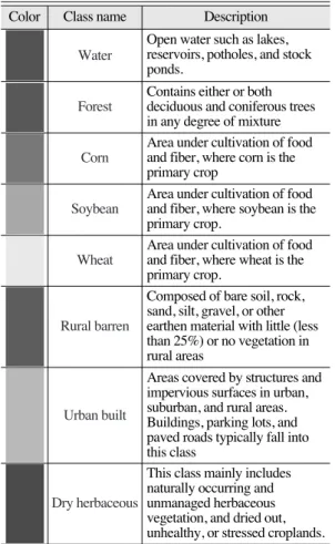
and dry herbaceous. Each class has a specific color.
Table 2 shows land use classes and their description.
Support vector machine and spectral angle mapper classification methods were followed. ENVI v4.5
software was used to carry out the two classifications methods.
3. Support vector machine (SVM)
Support vector machine gives good classification result and it is very useful technique for image classification (Hsu et al., 2007). In this section we give a very brief introduction to SVM’s.
Let (xi, yi)1≤i≤nset of training examples, each example xi∈Rn, n being the dimension of the input space, belongs to a class labeled by yi∈{-1, 1}. Our aim is to find a hyperplane which divides the set of example such that all the points with same label are on the same side of the hyperplane (Chapelle, 1999). The hyperplane separating two classes can be defined as:
H: w_·x_- b = 0 (1) where w_is normal vector of the hyperplane H, x_is an input vector. Support vectors are the vectors that are close to the boundary of two classes. The support vectors of each class define additional hyperplane H1 and H2 (eq 2) that are parallel to separating hyperplane H.
H1: w_·x_- b = +1
H2: w_·x_- b = -1 (2) The hyperplane decision function can be written as:
sng(w_·x_- b) (3) To find the hyperplane H that is in maximum distance from hyperplanes H1 and H2 containing support vectors Lagrange’s multipliers method is used and object can be amounted to the minimization of the following function:
F(w, b, a) = Sni=1Snj=1∝i∝jyiyj_x
i_x
j-
Si=1n ∝i (4) 1
2 Fig. 2. Flight line 11 and 12 of Little Miami River watershed
image used in classification a) Flight line 11, b) Flight line 12.
Table 2. Land use image classes and description Color Class name Description
Water
Forest
Corn
Soybean
Wheat
Rural barren
Urban built
Dry herbaceous
Color Class name Description
Open water such as lakes, reservoirs, potholes, and stock ponds.
Contains either or both deciduous and coniferous trees in any degree of mixture Area under cultivation of food and fiber, where corn is the primary crop
Area under cultivation of food and fiber, where soybean is the primary crop.
Area under cultivation of food and fiber, where wheat is the primary crop.
Composed of bare soil, rock, sand, silt, gravel, or other earthen material with little (less than 25%) or no vegetation in rural areas
Areas covered by structures and impervious surfaces in urban, suburban, and rural areas.
Buildings, parking lots, and paved roads typically fall into this class
This class mainly includes naturally occurring and unmanaged herbaceous vegetation, and dried out, unhealthy, or stressed croplands.
where 0≤∝i≤C ∀i and Si=1n ∝iyi= 0 (5)
The complete classification of two sets of vectors is not possible. That is why C parameter is used for presenting penalty in the situation when points are situated between hyperplanes H1 and H2. This parameter is chosen by the user, a larger C corresponding to assigning a higher penalty to errors (Chapelle, 1999). The bigger value of C causes the better fitting of hyperplane to the training set (Urszula, 2005).
In case of non-linear separating, vectors are transformed to higher dimension space using a transformationf(x), where the vectors can be linearly separated. In this case function F (eq 4) formed as the follow:
F(w, b, a) = ∝i∝jyiyjf(x_
i) f (x_
j)
Si=1n ∝i (6) Knowing that the dot product in this equation can be substituted by kernel function K(xi, xj) the function F (eq 6) can have following form:
F(w, b, a) = Sni=1Snj=1∝i∝jyiyjK( x_i_xj) - Si=1n ∝i (7)
The ENVI SVM classifier provides four types of kernels: linear, polynomial, radial basis function (RBF), and sigmoid. The default is the radial basis function kernel, which works well in most cases. The mathematical representation of radial basis function is presented below.
K(xi, xj) = exp(-g||xi, xj||2), g > 0 (8) SVM is based on the statistical learning theory (ENVI, 2005) and it is time-consuming with the high resolution images.
ENVI’s SVM classification performs hierarchical classification process reducing image resolution.
Reduced-resolution improves classification
performance and it does not affect classification result significantly (ENVI, 2005). The hierarchical classification procedures are as follows:
Resampling the images into low resolution level Resampling the region of interest (ROI) to same resolution level
SVM classifier trains low resolution image and ROI.
In the training step, SMV trains each level of resolution, because training for each resolution level gives more accuracy.
Checking image values that exceed reclassification probability threshold.
In the next step, SVM examines the next higher resolution pyramid level, but excluding pixels that are marked as classified in the previous lower resolution level.
Above steps iterates until the highest resolution level of image.
4. Spectral angle mapper (SAM)
SAM permits rapid mapping of the spectral similarity of image spectra to target spectra (Kruse, 1999). This classification method uses n-dimensional angle and computes a spectral angle between each pixel spectrum and each reference (target) spectrum.
The smaller spectral means that pixel and target spectra are more similar (Shippert, 2003). Comparing spectral angle between these two spectra is not sensitive in illumination because changing illumination does not change the direction of the vector (ENVI, 2005). The pixels that have angle more 1
2
Sn j=1
Sn i=1
1 2
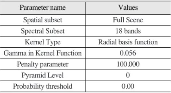
Table 3. Classification parameters for SVM classifier
Parameter name Values
Spatial subset Full Scene
Spectral Subset 18 bands
Kernel Type Radial basis function Gamma in Kernel Function 0.056
Penalty parameter 100.000
Pyramid Level 0
Probability threshold 0.00
Parameter name Values
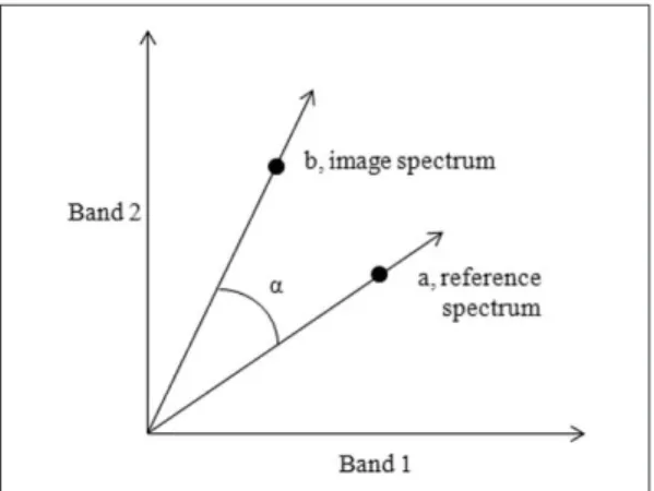
than specified threshold in radians are not classified (ENVI, 2005). A simplified representation to explain how the angle between a reference and an image spectrum from two-band data represented on a two- dimensional plot as two points obtained from image data (Park, 2007). The lines connecting each spectrum points (a, b) and the origin contain all possible positions for the sample, corresponding possibly intensity changes due to the illumination variability (Figure 3). The spectral angle (a) between two vectors is independent of their lengths (Park, 2007). This spectral between these two vectors, can be calculated by the following equation (9).
a = cos-1
( )
(9)SAM classifier was processed with the following parameters (Table 4).
Classification used single threshold for all classes.
Value is 0.100 and given in radians. This is the maximum angle between the end member spectrum
vector and the pixel vector. ENVI’s SAM classifier does not classify the pixels that have an angle larger than this threshold value (ENVI, 2005).
1) Ground truthing and testing points Ground truthing was carried out in 154 locations and the locations were marked. Ground truthing points are described in polygon shapes, which range from 5 to 929 pixels. Figure 4 shows one example of ground truthing point in soybean area.
2) Accuracy assessment
The accuracy assessment was based on whether the majority of classed pixels in a 3×3 pixel window, centered on a ground truth site, agreed or not. Thus, if five or more pixels were classified as corn, and ground truth indicated corn, then the majority criterion was satisfied and “corn class”
would be considered correct for that site.
Accuracy check was carried out in 200 testing points to estimate the accuracy of each classification (Table 5 and 6). The accuracy testing points were distributed randomly in the classified image. Once all of testing points were checked, the producer and user accuracy of the individual class as well as the overall accuracy of the classification were calculated. Using the data in Table 5 and 6, user and producer accuracy percentages can be calculated for each class separately, as given in Table 7 (Jensen, 1996). The (a→*b→)
||a→||*||b→||
Fig. 3. Vector presentation of a reference and image spectrum for a two band image.
Fig. 4. An example of ground truthing point in soybean area
Table 4. Classification parameters for SAM classifier
Parameter name Values
Spatial subset Full Scene
Spectral Subset 18 bands
Maximum angle (radians) Single value (0.100)
Parameter name Values
Kappa statistics for each classification was also calculated (Table 7).
The variance of Kappa can be calculated as follows:
sK2=
(
++
)
(10)where
T = ; W =
V = ; U =
where
N = total number of ground truthing points Xii= number of correct classification in the
specified class
Xi+= row total in error matrix for specified the class
X+i= column total in error matrix for the specified class
Using the Equation 10 and data in Table 5 and 6, Kappa (KHAT) variance can be calculated for each classifier as follows.
s2(KSVM) = 0.002217 for SVM classifier s2(KSAM) = 0.001829 for SAM classifier
Kappa statistics is often used to compare the results of multiple classifications (Congalton 1991). Kappa and its variance s2(K) have calculated for each classifier. Using these two statistics, a test statistic (Table 8) is calculated as follows:
Z = (11)
This test statistic follows as Gaussian (normal) distribution and can be used to determine whether
K1-K2
s2
K1 sK22 S xi + x+i
N2 S [xii (xi + x+i)]
N2
S S [xij (xj + x+i)]
N3 S xii
N
(1_T)2(W_4U)2 (1_U)4
2(1_T)(2TU_V) (1-U)3 T(1_T)
(1-U)2 1
N
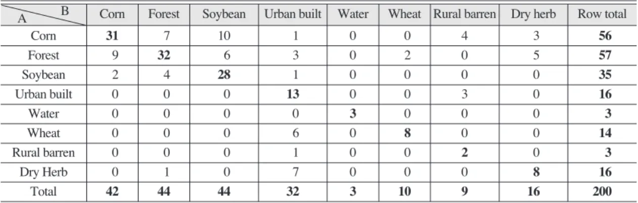
Table 5. Accuracy assessment table for support vector machine classification. A: Classified, B: Reference
A B Corn Forest Soybean Urban built Water Wheat Rural barren Dry herb Row total
Corn 31 7 10 1 0 0 4 3 56
Forest 9 32 6 3 0 2 0 5 57
Soybean 2 4 28 1 0 0 0 0 35
Urban built 0 0 0 13 0 0 3 0 16
Water 0 0 0 0 3 0 0 0 3
Wheat 0 0 0 6 0 8 0 0 14
Rural barren 0 0 0 1 0 0 2 0 3
Dry Herb 0 1 0 7 0 0 0 8 16
Total 42 44 44 32 3 10 9 16 200
A B Corn Forest Soybean Urban built Water Wheat Rural barren Dry herb Row total
Table 6. Accuracy assessment table for spectral angle mapper classification. A: Classified, B: Reference
B A Corn Forest Soybean Urban built Water Wheat Rural barren Dry herb Row total
Corn 41 3 3 2 0 0 1 7 57
Forest 4 28 13 0 0 0 0 3 48
Soybean 0 1 39 0 0 0 0 0 40
Urban built 0 0 0 6 0 0 4 0 10
Water 0 0 0 0 6 0 0 0 6
Wheat 0 0 0 1 0 5 1 1 8
Rural barren 0 0 0 1 0 3 5 2 11
Dry Herb 0 4 0 2 1 1 4 8 20
Total 45 36 55 12 7 9 15 21 200
A B Corn Forest Soybean Urban built Water Wheat Rural barren Dry herb Row total
difference between the two classifications is significant or not. Significance at 95% is obtained by comparing the Z-score to the equivalent value (1.96) from the normal tables. If the Z-score is greater than 1.96, the classification accuracy results are significantly different (Table 8). The normal tables can also be used to test significance at other levels (e.g., 90%, 99%) as desired.
5. Results and Discussion
SAM was found to produce more accurate classification (69.0%) than SVM (62.5%) (Table 7).
However, both classification results were low. Major factor caused the accuracy to be lower is that study area is very complicated itself. Urban and rural areas mixed together in the study area. That makes difficult to divide the study area into two pieces which are urban and rural. In the similar studies that are cited in the manuscript, usually unmixed images were used for classification. Therefore, classification result was higher. For instance, Liu et al., (2006) tested SVM and SAM classifier in only urban area which is taken over the Washington, DC mall. Xiaomei et al., (2009)
evaluated the response of both classifiers to noises and uncertainty in original hyperspectral image of rural area. Also, few classes were included (dry herbaceous and rural barren) which are very complicated to be classified well. Dry herbaceous area is similar to urban built area in terms of spectral information and color code. Hence, dry herbaceous area was not classified well. According to the accuracy assessment table, more than 50% of dry herbaceous area was misclassified as other classes (especially as urban area). Also dry herbaceous is located on the agricultural area mixed with single signature and it is the dried part of agricultural area.
Some area which has little dry herbaceous, mostly misclassified as dry herbaceous class.
In both classifications the water category was classified well with similar user accuracies. In the case of forest, the user and producer accuracies of SAM were better (58.3, 77.8%) than SVM (56.1, 72.7%) respectively.
As far as agriculture crops are concerned, user and producer accuracies of corn and soybean were better in SAM than SVM. But, wheat was classified with 80.0% producer accuracy in SVM which is better than SAM with 55.6%. In the case of user accuracy of wheat, SAM classified better (62.5%) than SVM (57.1%) and in the case of wheat it was vice versa (Table 7). In case of dry herbaceous, user and producer accuracies were same (50.0%) and better than SAM (40.0, 38.1%).
SVM classified the remaining two classes (rural barren and urban built) with higher percentage of user accuracies than SAM. But SAM classified with high percentage of producer accuracies than SVM in these classes. Among the 8 classes, only water was classified with more than 80% user and producer accuracy in both classifications. Rural barren in SAM and SVM, dry herbaceous in SAM were classified with less than 40% producer accuracy. Rural barren and dry Table 7. Accuracy assessment values for SVM and SAM
classification
Classes Accuracy of SVM Accuracy of SAM User Producer User Producer
Corn 55.4% 73.8% 71.9% 91.1%
Forest 56.1% 72.7% 58.3% 77.8%
Soybean 80.0% 63.6% 97.5% 70.9%
Urban built 81.3% 40.6% 60.0% 50.0%
Water 100% 100% 100% 85.7%
Wheat 57.1% 80.0% 62.5% 55.6%
Rural barren 66.7% 22.2% 45.5% 33.3%
Dry Herb 50.0% 50.0% 40.0% 38.1%
Overall accuracy Overall accuracy
Accuracies = 62.5% = 69.0%
Kappa = 0.54 Kappa = 0.62 Classes Accuracy of SVM Accuracy of SAM
User Producer User Producer
herbaceous in SAM were classified with less than 50%
user accuracy. Overall, SAM performed well compared to SVM in Kappa statistics also (Table 7).
According to accuracy analysis, SAM classified better for a single signature such as corn, soybean and wheat area. Especially for corn and soybean, SAM performed much better than SVM (Fig. 5 and 6).
Whereas, SVM classified single signature area mixed with other classes such as soybean, forest and dry herbaceous. For both classifiers, forest area was mixed with soybean and corn area, since spectral and color code are similar.
However, SVM was better for classes of mixed signatures such as urban built, rural barren and dry herbaceous area (Fig. 7, 8 and 9). Naturally, dry herbaceous and rural barren areas exist with forest and agriculture. Urban built area is one of the most difficult classes to classify accurately when it is located along with forest. SAM misclassified such mixed areas in some area (Fig. 8).
Shadow is very particular case, since it is not a single class. Mostly, SAM gave better classification in areas with shadow effects than SVM. In some areas, SAM misclassified shadows, while SVM classified as water or soybean.
From the Table 7, overall accuracy of SAM is
more than SVM. It appears that using spectral information in image classification shows more accurate result. Some studies proved that using spectral knowledge into multispectral classification yields better results (Mercier, 2003).
Kappa is the statistical measure of inter-rate agreement for qualitative assessment in classification accuracy. The kappa statistics shows that both classifiers have performed well. However, the SAM (0.62) classifier shows little bit better result than SVM (0.54). In case of SAM, it gives substantial agreement, whereas SVM performed with moderate agreement in accuracy of classification.
Hypothesis test was calculated for comparing the results of two classifiers (Table 8). This test produces Fig. 5. Portion of corn area. a) Image of study area b) Image
classified by SVM c) Image classified by SAM.
a b c
Fig. 6. Portion of soybean area. a) Image of study area b) Image classified by SVM c) Image classified by SAM.
a b c
Fig. 8. Portion of rural barren area. a) Image of study area b) Image classified by SAM c) Image classified by SVM.
a b c
Fig. 9. Portion of dry herbaceous area. a) Image of study area b) Image classified by SAM c) Image classified by SVM.
a b c
Fig. 7. Portion of urban built area. a) Image of study area b) Image classified by SAM c) Image classified by SVM.
a b c
Table 8. Hypothesis test for comparing two classification results Classifier Kappa Kappa variance Z-score
SVM 0.54 0.002217
1.2574
SAM 0.62 0.001829
Classifier Kappa Kappa variance Z-score
the difference between the two classifications. From the Table 8, Z-score is less than 1.96, consequently two classification accuracy results are not significantly different.
6. Conclusion
Classification of hyper spectral high resolution image based on two classification (SVM and SAM) algorithms was tested for their suitability. Based on the results, SAM is found to classify more accurately than SVM. As far as processing time is concerned, SAM produces outputs sooner than SVM. These conclusions are based on the present study. Therefore further studies are needed to ascertain these findings with diverse images from other satellites and many land use classes.
References
Chapelle O., P. Haffner, and V.N Vapnil, 1999.
Support Vector Machines for Histogram- Based Image Classification, Neural Networks, IEEE Transactions on, 10: 1055-1064.
Choen K., and C. Seonghoon, 1996. Spectral Angle Mapper Classification and Vegetation indices Analysis for winter cover monitoring using JERS-1 OPS data, Geoscience and Remote Sensing Symposium, IGARSS ‘96. Remote Sensing for a Sustainable Future. 4: 977-1979.
Congalton, R. G., 1991. A review of assessing the accuracy of classifications of remotely sensed data, Remote Sensing of the Environment, 37: 35-46.
Girouard G, A. Bannari, A. El Harti, and A. Desrochers, 2004. Validated Spectral Angle Mapper Algorithm for Geological Mapping:
Comparative Study between Quickbird and Fig. 10. a) High resolution image of study area.
(Bands: 2, 5, 11 in BGR)
b) Classification result by SAM classifier c) Classification result by SVM classifier a
b
c
Landsat-TM, The 20th International Society for Photogrammetry and Remote Sensing Congress, Geo-Imagery Bridging Continents, 599-605.
Hsu, C. W., Chang, C. C., and C. J. Lin, 2008. A Practical Guide to Support vector Machine, Department of Computer Science National Taiwan University, Taipei 106, Taiwan, 1.
Janssen L. F. Lucas, 2000. Principles of Remote Sensing, ITC educational textbook series 2, International Institute for Aerospace Survey and Earth Science, Netherland, p. 141.
Jayakumar, S., A. Ramachandran, L. Jung Bin, and J.
Heo, 2007. Object-oriented classification and QuickBird multi-spectral imagery in forest density mapping, Korean journal of remote sensing, 23: 153-160.
Jensen J. R., 1996. Introductory Digital Image Processing, A Remote Sensing Perspective, 2nd edition, Prentice Hall, New Jersey.
Kruse, F. A., A. B. Lefkoff, J. B. Boardman, K. B.
Heidebrecht, A. T. Shapiro, P. J. Barloon, and A. F. H. Goetz, 1993. The Spectral Image Processing System (SIPS) - Interactive Visualization and Analysis of Imaging spectrometer Data, Remote Sensing of the Environment, 44: 145-163.
Liu., Z, D. Li, and Q. Qin, 2006. Partially Supervised Classification: Based on Weighted Unlabeled Samples Support Vector Machine, International Journal of Data Warehousing & Mining, 2: 42-56.
NCEA, 2006. Classification of high spatial resolution, Hyperspectral remote sensing imagery of the Little Miami River watershed in Southwest Ohio, USA, National Centre for Environmental Assessment, U.S. Environmental Protection Agency, Cincinanati, OH, Project Report.
Oliver, C., P. Haffner, and V. N. Vapnik, 1999.
Support vector machines for histogram-based
image classification, IEEE Transactions on Neural Networks, 10: 1055-1064.
Park B., W. R. Windham, K. C. Lawrence, and D. P.
Smith, 2007. Contaminant Classification of Poultry Hyperspectral Imagery using a Spectral Angle Mapper Algorithm, Biosystems Engineering Journal, 96: 323-333.
ENVI 2005. ENVI v4.5, IDL Assistance v1.0, Research Systems., INC.
Shippert, P., 2003. Introduction to Hyperspectral Image Analysis, Online Journal of Space Communication, downloaded on Jan 2009 from URL: http://satjournal.tcom.ohiou.edu/
pdf/shippert.pdf
Urszula M. K. and P. Kubacki, 2005. Support Vector Machines in Handwritten Digits Classification, Proceedings of the 2005 5th International Conference on Intelligent Systems Design and Applications (ISDA’05), 406-411.
Yonezawa, C., 2007. Maximum likelihood classification combined with spectral angle mapper algorithm for high resolution satellite imagery, International Journal of Remote Sensing, 28: 3729-3737.
Mercier, G. and M. Lennon, 2003. Support vector machines for hyperspectral image classification with spectral-based kernels, Geoscience and Remote Sensing Symposium, IEEE International, 1: 288-290.
Xiaomei., W, D. Peijun, T. Kun, and L. Guangli, 2009. Impacts of noise on the results hyperspectral remote sensing image classification - Performance evaluation of support vector machine classifier, Science paper Online. Accessed from http://www.
paper.edu.cn/en/paper.php?serial_number=20 0903-517 on May 2009.