Mean Square Response Analysis of the Tall Building to Hazard Fluctuating Wind Loads
Jong Seop Oh* , Eui Jin Hwang**, and Ji Hyeob Ryu***
재난변동풍하중을 받는 고층건물의 평균자승응해석
오종섭*·황의진**·류지협***
(접수일자: 2013년 10월 3일/심사완료일: 2013년 12월 3일)
ABSTRACT Based on random vibration theory, a procedure for calculating the dynamic response of the tall building to time-dependent random excitation is developed. In this paper, the fluctuating along- wind load is assumed as time-depen- dent random process described by the time-independent random process with deterministic function during a short dura- tion of time. By deterministic function A(t)=1-exp(-βt), the absolute value square of oscillatory function is represented from author’s studies. The time-dependent random response spectral density is represented by using the absolute value square of oscillatory function and equivalent wind load spectrum of Solari. Especially, dynamic mean square response of the tall building subjected to fluctuating wind loads was derived as analysis function by the Cauchy’s Integral Formula and Residue Theorem. As analysis examples, there were compared the numerical integral analytic results with the analy- sis fun. results by dynamic properties of the tall uilding.
KEYWORDS oscillatory function, response spectral density function, Cauchy’s Integral Formula, residue theorem
요 약 시간과 공간에 따라 변화하는 난류성분의 변동풍하중을 받는 고층건물의 경량화 및 연성화 현상은 고유진동수와 감 쇠비를 적게함으로서 동적으로 매우 불리한 진동문제을 발생하게 되어, 변동풍하중을 받는 도심의 고층건물에 대한 동적해 석의 중요성이 인식되고 있다. 본 논문에서는 돌풍과 같이 짧은 시간동안에 통계적 성질이 변화하는 변동풍하중을 나타내기 위하여 정상불규칙 풍하중에 시간에 따라 변화하는 결정적함수(A(t) = 1-exp(-
β
t))를 곱하여 나타냈고, 이러한 변동풍하중을 받는 고층건물에 대한 평균류방향의 동적변위응답해석은 진동이론으로부터 Time-dependent Response Spectral Density함수 를 나타냈고, 진동함수를 포함하여 나타내는 Time-dependent Response Spectral Density의 진동수영역에 대한 적분의 해로부 터 동적응답을 해석적으로 구하기 위하여 Contour적분에서 Cauchy의 적분정리와 잔유치 정리(residue theorem)에 의한 잔유 치 적분으로부터 해석함수를 구했다. 해석 예에서 본 논문에서 구한 해석함수와 기존의 수치해석방법에 따른 결과를 비교 검토했고, 고층건물의 동적 특성에 따른 해석결과도 비교 검토했다.핵심용어 진동함수, 응답스펙틀럴 함수, 코시 적분정리, 잔유치정리
1. INTRODUCTION
In recent years application of advances in structural materials, structural design, innovative architectural concepts, and new construction me thods has resulted in flexible and
lighter tall building with reduced damping. Consequently, their vulnerability to random effects has been escalated.
Thus, in serviceability designing these tall building systems efficiently for random excitation including time-dependent properties such as wind and earthquake, it is important to know how to estimate the time-dependent random response in a specified duration of such loading. The time-dependent
*한려대학교 건축공학과, 교수(E-mail: [email protected])
**정회원, 한려대학교 토목환경공학과 교수
***정회원, 한려대학교 토목환경공학과 교수
random processes are modeled as a uniformly modulated random process based on Corotis and Vanmarcke (1975), Hammond (1968), Nigam (1983). That is, the time-dependent random excitation can be expressed as a product of a time- independent random excitation process with a deterministic function.
In 1961, Davenport first applied statistical concepts to fluctuating wind load on structures. Since that time, the statistical approach is the basis for design method of tall building subjected to fluctuating wind load. However since past decades, although it has been recognized that random fluctuating wind excitations are including time-dependent random processes during a short duration of time such as instantaneous gust wind, in computing the overall response of tall building subjected to fluctuating wind load, it is commonly limited that random wind excitation can be described by a stationary process for mean wind load of long time wind Davenport (1962), Simiu (1974, 1976), Solari (1988, 1993). Of course, these analysis methods may be considered a possible design method in engineering field, but it is important that the design process of serviceability can be considered to be a response properties during a short duration of time such as instantaneous gust wind. Until now, there are no the alongwind and the acrosswind analysis methods of the tall building subjected to fluctuating random wind loads. Thus, in the base step of research, the main purpose of this paper is to present on alongwind timedependent response of tall building subjected to fluctuating random wind load during a short duration of time.
Based on random vibration theory, a procedure for calculating the dynamic response of the tall building to time-dependent random excitation is developed. In this paper, the fluctuating wind load is assumed as time-dependent random process described by the time-independent random process with deterministic function during a short duration of time. By deterministic function A(t)=1-exp(-βt), the absolute value square of oscillatory function is represented from author’s studies. The time-dependent random response spectral density is represented by using the absolute value square of oscillatory function and equivalent wind load spectrum of Solari. Especially, dynamic mean square response of the tall building subjected to fluctuating wind loads was derived as analysis function by the Cauchy’s Integral Formula
and Residue Theorem. As analysis examples, there were compared the numerical integral analytic results with the analysis function results by dyn- amic properties of the tall building.
2. HAZARD FLUCTUATING WIND LOAD
2.1 Fluctuating wind velocity spectrum
Dynamic alongwind response of tall building subjected to random alongwind load is mainly due to turbulent velocity fluctuation in the atmospheric boundary layer. Such fluctuating velocity may be caused by a superposition of eddies, characterized by a periodic motion of frequency. So the total kinetic energy of the turbulent motion may be regarded as a sum of contributions by each of the eddies of the flow.
That is, fluctuating wind velocity spectrum representing the dependence upon wave number of these energy contributions is defined as the energy spectrum of the turbulent motion.
Among them, the representative spectrum used for structural design purpose is given as follows
(1) (2) where the Eq. (1) by Davenport (1961), the Eq. (2) by Solari (1987), x = 1200 n/ , f = nz (z), = mean wind velocity at height 10 m, u
*= shear velocity, n = frequency,
(z) = mean wind velocity at height z.
2.2 Fluctuating wind load spectrum
If the horizontal dimensions of the body are small compared to the scale turbulence, it is reasonable to assume that the fluctuating pressures are given by the formulas.
(3) (4) where P
w=windward fluctuating pressure, P
l=lee ward fluctuating pressure; C
w, C
l=mean pressure coefficient on the windward and leeward face of the structure, u(z)=
fluctuating wind velocity, q=air density. From alongwind cross-correlation functions of Eq. (3) and Eq. (4), the cross spectrum of the fluctuating pressure can be expressed as
nS
u( z n , )/u
*2= 4.0x
2/ 1 ( + x
2)
4/3nS
u( z n , )/u
*2= 266f/ 1 58.7 f ( + )
5/3U
10U U
10U
P
w= C
wqU z ( ) u z ( )
P
l= C
lqU z ( ) u z ( )
follows
(5) At above fluctuating pressure assumed as a distributed stationary random load, alongwind fluctuating wind load spectrum can be expressed as (Simiu 1996).
(6) where
=mode shape at points
=mean wind velocity
=fluctuating velocity spectrum
=coherence function N(n)=alongwind cross-correlation coefficient
And recently, Solari (1993) published power spectral density (fluctuating wind load spectrum) of the first fluctuating modal force based on reduced equivalent wind spectrum Solari (1988) as follows
(7) where
= reduced equivalent wind spectrum
σ
u(z) = standard deviation of alongwind turbulence C
D= C
w+ C
l= drag coefficient, τ = averaging time H,B and h = height, depth, and equivalent height K
b= nondimensional quantity defined by mean velocity profile.
3. DYNAMIC RESPONSE ANALYSIS
3.1 Time-dependent spectral density function In many applications, the time-dependent power spectral density function of random process can be shown based on random vibration theory Nigam (1983, 1994). The time-dependent random process is assumed to be a uniformly
modulated process, it can be expressed by Stieltjes inte- gral form as follows
(8) (9)
where A(t) = slowly varying deterministic function of, X(t) = time-independent (stationary) random processes. That is, X(t) and covariance function K(t
1, t
2) of a random pro- cess defined by X(t) can be expressed as
(10)
(11)
In the Eq. (11), from defined by generalized power spec- tral density to the function can be defined as follows
(12) Since X(t) is time-independent (stationary), by writing, t
2= t
1+ τ, autocorrelation function R(τ) can be expressed as
(13)
(14) where Φ(w) is the power spectral density function δ(w
2− w
1) is the Dirac delta function. From Eq. (11), under this assumption, A(t) = 1 then Y(t) = X(t).
The autocorrelation function of Y(t) is given as follows
(15) In the Eq. (15), from Eq. (14) and the property of the Dirac delta function, It may also be expressed as
(16)
In the Eq. (16), the mean square value of is obtained by setting t
1= t
2= t, as follows
(17) S
p1 p2,( ) ρ n =
2C
p( )C z
1 p( )U z z
2( )S
1 u11/2( z
1, n )
S
u21/2( z
2, n )Coh y (
1, , , , y
2z
1z
2n )N n ( )
S
f( ) n ψ
i( ) z
1o
∫
H o∫
H o∫
B o∫
Bψ
j( )U z z
2( )U z
1( )S
2 u11/2( z
1, n )
=
S
u21/2( z
2, n )Coh y (
1, , , , y
2z
1z
2n )N n ( )dz
1dy
1dy
2ψ
i( ) ψ z
1,
j( ) z
2U z ( ) U z
1, ( )
2S
u1( z
1, n ) S ,
u2( z
2, n ) Coh y (
1, , , , y
2z
1z
2n )
S
f11( ) n = ρBHC
DU h ( )σ
u( )K h
b2S
ueq*( )χ n;τ n ( )
S
ueq*( ) n
χ n;τ ( ) sin
2( nπτ ) ( nπτ )
2--- x 1 , ( = for nπτ 0 = )
=
Y t ( ) A t = ( )X t ( )
Y t ( ) A t ( )e
–iwtd S w ( )
∞ –
∫
∞=
X t ( ) e
–iwtd S w ( )
∞ –
∫
∞=
K t (
1, t
2) e
i w( 2t2–w1t1)E S w [ d ( ) S
1d
*( ) w
2]
∞ –
∫
∞∞ –
∫
∞=
Φ′ w (
1, w
2)dw
1dw
2= E S w [ d ( ) S
1d
*( ) w
2]
R τ ( ) e
i w( 2(t1+τ) w– 1t1)E S w [ d ( ) S
1d
*( ) w
2]
∞ –
∫
∞∞ –
∫
∞=
E S w [ d ( ) S
1d
*( ) w
2] Φ w = ( )δ w
1(
2– w
1)dw
1dw
2K
YY( t
1, t
2) A t ( )A
1 *( ) t
2∞ –
∫
∞∞ –
∫
∞=
e
i w( 2t2–w1t1)E S w [ d ( ) S
1d
*( ) w
2]
K
YY( t
1, t
2) A t ( )A
1 *( )e t
2 iw t(2–t1)Φ
XX( ) w w d
∞ –
∫
∞=
σ
Y2( ) t A t ( )
2Φ
XX( ) w w d
∞ –
∫
∞=
(18)
(19) Eq. (19) represents the time-dependent spectral distribu- tion of average energy as a function of time and is the power spectral density function of the time-independent (sta- tionary) random process
3.2 Dynamic response of MDOF
The dynamic response of tall building subjected to distributed random excitation can be estimated using random vibration theory in either frequency or time domain. In this paper, the dynamic response of the coupled MDOF system is obtained by using normal mode method described by a frequency domain. The equations of motion of the coupled MODF with a described lumped mass system can be expressed as
(20) where M,C,K=mass, damping, and stiffness matrices of the system, F(x)=external force. Using the normal mode within the Eq. (20), the equation of uncoupled MDOF system can be expressed as
(21) where q
i, ξ
i, w
i=generalized coordinate, damping ratio, and natural frequency in the ith, M
i, F
i(t)=generalized mass and external force in the ith mode, ψ
i(z)=the ith mode shape at height z, m(z), p(z, t)=the mass of the structure and the external force per unit length.
In the Eq. (21), the dynamic response of the time- invariant uncoupled MDOF system subjected to time- dependent random processes can be obtained in the frequency domain. From concepts of the Eq. (9) the input and the output processes may be written as
(22)
(23)
(24) Then, from the orthogonal properties of Eq. (22) and the applications of Eq. (8)-(19), the timedependent response spectral density function for the Eq. (21) can be expressed as follows
(25)
(26) where integral term is a time-independent (stationary) ran- dom process and G
j(t, w) is a oscillatory function with deterministic function A(t). In the Eq. (25), if the damping is small and resonant peaks are all separated, the cross terms become negligible and can be rewritten as
(27)
Also, from associated with Eq. (21), (22) and Eq. (24), the oscillatory function included within time-dependent response spectral density function of uncoupled MDOF system can be obtained by differe- ntial equation as fol- lows
(28)
where , , . In this paper, using A(t) = (1-e
-βt) and β is a constant
associated with amplitude. The solutions of Eq. (28) can be derived by assumed as the general solution G
h(t,w) = Ae
λt, the particular solution G
p(t,w) = k
1+k
2e
-βtand initial conditions G(0,w) = 0, G(0,w) = 0.
Thus, from the solution of Eq. (28), the oscillatory function G
i(t,w) can be obtained by author as follows
G
i(t,w) = (29)
Φ
YY( t w , ) w d
∞ –
∫
∞=
Φ
YY( t w , ) = A t ( )
2Φ
XX( ) w
Mx·· Cx· Kx + + = F t ( )
M
i( q··
i+ 2ξ
iw
iq·
i+ w
i2q
i) F =
i( ) x
x t z ( ) , e
iwtd X z w ( , )
∞ –
∫
∞=
ψ
i( ) x G
i( t w , )e
iwtd Q
i( ) w
∞ –
∫
∞ i 1=∑
∞=
q
i( ) t G
i( t w , )e
iwtd Q
i( ) w
∞ –
∫
∞=
F
i( ) t ψ
i0
∫
H( )e z
1 iwtA t ( ) P z d (
1, w ) d z
1∞ –
∫
∞=
s
x( t z w , , ) ψ
i( )ψ z
j( )G z
i( t w , )G
j*( t w , ) Z
i( )Z w
j*( ) w ---
j 1=
∑
∞ i 1=∑
∞=
ψ
i0
∫
H( )ψ z
1 j( )s z
2 Ps( z
1, , z
2w ) z d
1d z
2 0∫
HZ
i( ) M w =
i( w
io2– w
2+ 2iξ
iww
io)
s
x( t z w , , ) ψ
i( ) z
2G
j( t w , )
2Z
i( ) w
2---
i 1=
∑
∞=
ψ
i0
∫
H( )ψ z
1 j( )s z
2 Ps( z
1, , z
2w ) z d
1d z
2 0∫
HG ··
i
2G ·
i
( iw ξ +
iw
io) G
i( w
io2– w
2+ 2iξ
iww
io)
+ + =
A t ( ) w (
io2– w
2+ 2iξ
iww
io) G ··
i
G ·
i
( t w , )
= G ·
i
G ·
i
( t w , )
= G
i= G
i( t w , )
2iw
idA B – – C
[ ]
2iw
idV
2---
where
Also, because the fluctuating alongwind load spectrum of integral term within the Eq. (27) can be expressed as simplified formulation Eq. (7), the time-dependent response spectral density function in the fundamental mode of tall building subjected to the time-dependent random wind load defined such as Eq. (8) and (9) can be obtained from Eq. (7), (27) as follows
(30)
In this paper, the oscillatory function’s absolute value square of Eq. (30) can be obtained by author as follows
+
+ }
+ (31)
The parameters of the Eq. (31) can be seen by the appendix (a)
Thus, the mean square value for time-dependent displacement resopnse of the tall building subjected to the time-dependent random wind load can be written by Eq. (18), (30) as follows
(32)
3.3 Analysis function of Eq.(32)
In this paper, the integration solution of Eq. (32) can be evaluated by contour integration in a complex plane using the Cauchy residue theorem.
Eq. (32) can be tranformed in order to use Cauchy residue theorem as follows.
(33)
(34)
In the Eq. (33) and (34), z is height of the tall building, Z is complex function. The polynomial rearrange about ω in the Eq. (33) can be obtained as follows
(35)
The parameters of the Eq. (35) can be seen by the appendix (b). Again, from Eq. (33) and (35), let the f(ω) be replaced by the complex variable as follows
(36) where
w
id= w
io1 – ξ
i2A = ( V
2– V
1e
–βt) B = ( X
2V
2– V
1β )e
X1tC = ( X
1V
2– V
1β )e
X2tX
1= ( – iw – ξ
iw
io+ iw
id) X
2= ( – iw – ξ
iw
io+ iw
id) V
1= w
io2– w
2+ 2iξ
iww
ioV
2= β
2– 2 β iw ξ ( +
iw
io) + V
1s
x( t z w , , ) ψ
1( ) z
2G
1( t w , )
2M
12( w
102– w
2+ 2iξ
1ww
10)
2---S
f11( ) n
=
G
1( t w , )
2G
1( t w , )
2= 2w
2w
d– + w
2( 4β
2w
d+ 4w
o2w
d– 8βξw
ow
d) 2w ( –
d) {
+ 4βw (
d– 4ξw
ow
d2) + ( 2 β
2w
d+ 2w
o2w
d– 4βξw
ow
d)
2}
–1w
4{ Γ
122+ Γ
62exp ( – 2ξw
ow
d) }
[
w
2{ 2 Γ
11Γ
12+ I
132+ ( 2 Γ
5Γ
6+ I
72)exp 2ξw ( –
ot )}
Γ
112+ Γ
52exp ( – 2ξw
ot )
{ } { w
4( – 2Γ
12Γ
6exp ( – ξw
ot ) )
+ +
+w
2( 2Γ
13Γ
7– 2Γ
12Γ
5– 2Γ
11Γ
6)exp ξw ( –
ot ) 2Γ
11Γ
5exp ( – ξw
ot )
( – ) cos wt ( )
w
2( – 2 Γ
11Γ
7– 2 Γ
13Γ
5)exp ξw ( –
ot )) {
+
w
4( – 2Γ
12Γ
7– 2Γ
13Γ
6)exp ξw ( –
ot )}sin wt ( )]
σ
x2( ) t z , s
x( t z w , , ) w d
∞ –
∫
∞=
σ
x2( ) t z , s
x( t z w , , ) w d
∞ –
∫
∞=
f Z ( ) Z d
∫
c=
2 πi Res
1
=
∑
n( f Z ,
k)
=
Res f Z ( ,
o) 1 k 1 –
( )
--- d
k 1–dZ
k 1–---
Z
lim
→Zo( Z Z –
o)
kf Z ( )
=
σ
x2( ) t z , s
x( t z w , , ) w d
∞ –
∫
∞=
ψ
1ψ
2+ ψ
3+ ψ
4ψ
5ψ
6--- w d
∞ –
∫
∞=
f w ( ) ⇒ f Z ( ) ψ
2+ ψ
3+ ψ
4ψ
5ψ
6---
=
ψ
2= Z
4F Z +
2G H +
ψ
3= ( Z
4I Z +
2J K + )e
iZtψ
4= ( Z
2L Z +
4M )e
iZtψ
5= ( Z
4A Z +
2B C + )
ψ
3= ( Z
4+ Z
2D E + )
In the Eq. (36), the particular points can be evalualuated by
(37)
since the particular points of Eq. (37) are simple poles, thus, the effect particular points of unit circles can be evaluated by
(38) From Eq. (34), (36) and (38), the residue of the effect particular point can be evaluated by
Res (39)
where
From the similar process as Eq. (39), the residues of Z
2, Z
3, Z
4can be evaluated by
(40) The parameters of the Eq. (40) can be seen by the appen- dix (c). From Eq. (36), (39), and (40) can be evaluated by (41)
Thus, From Eq. (33) and (41), the mean square response analysis function of the Eq. (32)’s integration solution can be evaluated by author as follows
(42)
4. NUMERICAL EXAMPLE
The tall building model examined in this paper is located in the urban area. The properties of the tall building:
H = 250 m, B = 30 m, D = 30 m and of wind load: ρ = 1.125 kg/m
3, C
D= 1.3, C
Z= 10, C
y= 16, C
X= 1.54, σ
u(h) = 5.39 m/
s, τ = 0=0, K
b= 1.5, ω
u= ω
o*10, z
o= 0.07, u
*= 2.2 m/s, U(h) = 2.5u
*ln(h/z
0).
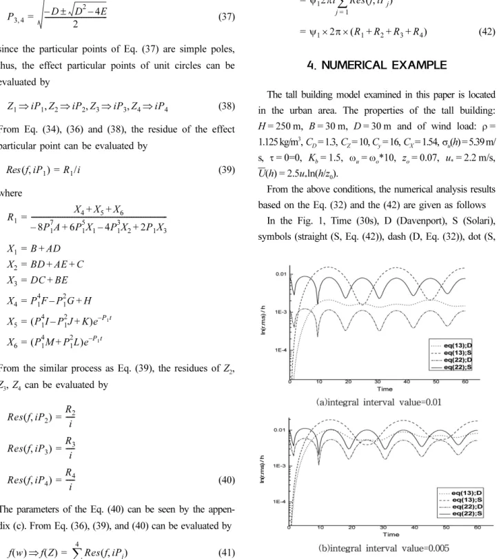
From the above conditions, the numerical analysis results based on the Eq. (32) and the (42) are given as follows
In the Fig. 1, Time (30s), D (Davenport), S (Solari), symbols (straight (S, Eq. (42)), dash (D, Eq. (32)), dot (S, Z = ± iP
1, ± iP
2, ± iP
3, ± iP
4P
1 2,– B ± B
2– 4AC --- 2A
=
P
3 4,– D ± D
2– 4E --- 2
=
Z
1⇒ iP
1, Z
2⇒ iP
2, Z
3⇒ iP
3, Z
4⇒ iP
4f iP ,
1( ) R =
1/i
R
1X
4+ X
5+ X
68P
17A
– + 6P
15X
1– 4P
13X
2+ 2P
1X
3---
=
X
1= B AD + X
2= BD AE C + + X
3= DC BE + X
4= P
14F P –
12G + H X
5= ( P
14I P –
12J + K )e
–P1tX
6= ( P
14M P +
12L )e
–P1tRes f iP ( ,
2) R
2--- i
=
Res f iP ( ,
3) R
3--- i
=
Res f iP ( ,
4) R
4--- i
=
f w ( ) ⇒ f Z ( ) Res f iP ( ,
j)
j 1=
∑
4=
σ
x2( ) t z , S
x( t z w , , ) w d
∞ –
∫
∞=
ψ
12πi Res f iP ( ,
j)
j 1=
∑
4=
ψ
1× 2π × ( R
1+ R
2+ R
3+ R
4)
=
Figure 1. Numerical analysis results of Eq. (32), (42).
Eq.32)), short dash dot (D, Eq. (42)).
From numerical analysis results of the Fig. 1, it shows that the mean square response of the Eq. (32) can be evaluated by the summation of a discrete integral interval value and the mean square response values are largely effected by integral interval values because the numerical analytic processes considered the different freq- uency range of the fluctuating wind load spectrum.
Thus, in order to obtain the function solution of the Eq.
(32), using the Cauchy residue theorem can be derived the analysis function such as the Eq. (42). From the Fig. 1(a), (b), it shows that mean square response analysis function of the Eq. (42) is very close to the Eq. (32) of the integral interval value 0.005.
5. CONCLUSION
In this paper, in order to provide the mean square response estimation method of a tall building subjected to the time-dependent random wind load as uniformly modulated process concept, the absolute value square of the oscillatory function for deterministic function could be derived, finally, the mean square response analysis function could be derived by the Cauchy’s Residue Theorem. As analysis examples, there were compared the numerical integral analytic results with the analysis function results by the dynamic proper- ties of the tall building. From Fig. 1 for the Eq. (42)’s numerical analysis resultes, we know that the effectiveness of the Eq. (42)’s mean square response analysis function drived in this paper are evidenced by the dynamic properties of the tall building subjected to the fluctuating wind loads.
Thus, the absolute value square Eq. (31) of the oscillatory function and the Eq. (42)’s mean square response analysis
function proposed in this paper may be used for the time- dependent response analysis at the preliminary design state of the tall building subjected to the hazard fluctuating wind loads.
REFERENCES
1. Corotis, R. B., and Vanmarcke, E. H. (1975), Time-dependent spectral content of system response. J. Eng. Mech., ASCE, 101(5), 623-636.
2. Davenport, A. G. (1961), The application of statistical con- cepts to the wind loading of structures. Proc. Ins. Civil Eng.
(London), 19(6480), 449-471.
3. Davenport, A. G. (1962), The response of slender, line-like structures to a gust wind, Proc. Ins. Civil Eng.(London), 23(6610), 389-408
4. Hammond, J. K. (1968), On the response of single and multi- degree of freedom system to nonstationary random excita- tions. J. Sound Viv., 7(3), 393-416.
5. Nigam, N. C. (1983), Introduction to random vib- rations. MIT Press, 49-219.
6. Nigam, N. C. (1994), Applications of random vibrations. Narosa Pub. House.
7. Simiu, E. (1974), Wind spectra and dynamic alongwind response. J. Str. Div., ASCE, 100(9), 1897-1910
8. Simiu, E. (1976), Equivalent static wind loads for tall building design. J. Str. Div., ASCE, 102(4), 719-737.
9. Simiu, E., et al. (1996), Wind effects on structures; fundamen- tals and application design. John Wiley & Sons, 3rd Ed., 33- 272.
10. Solari, G. (1987), Turbulence modeling for gust loading J. Str.
Eng., ASCE, 113(7), 1550-1569.
11. Solari, G. (1988), Equivalent wind spectrum techn iniq iq ue:
theory and applications. J. Str. Eng., ASCE, 114(6), 1303-1323.
12. Solari, G. (1993), Gust buffeting ii: dynamic alongwind response.
J. Str. Eng., ASCE, 119(2), 383-398.