Performance Comparison of Data Mining Approaches for Prediction Models of Near Infrared Spectroscopy Data
Seung Hyun Baek*
*Division of Business Administration, Hanyang University ERICA Campus
근적외선 분광 데이터 예측 모형을 위한 데이터 마이닝 기법의 성능비교
백 승 현*
*한양대학교 에리카 캠퍼스, 경영학부
요 약
본 논문에서는 주성분 회귀법과 부분최소자승 회귀법을 비교하여 보여준다. 이 비교의 목적은 선형형태를 보유한 근적외선 분광 데이터의 분석에 사용할 수 있는 적합한 예측 방법을 찾기 위해서이다. 두 가지 데이터 마이닝 방법 론인 주성분 회귀법과 부분최소자승 회귀법이 비교되어 질 것이다. 본 논문에서는 부분최소자승 회귀법은 주성분 회귀법과 비교했을 때 약간 나은 예측능력을 가진 결과를 보여준다. 주성분 회귀법에서 50개의 주성분이 모델을 생 성하기 위해서 사용지만 부분최소자승 회귀법에서는 12개의 잠재요소가 사용되었다. 평균제곱오차가 예측능력을 측 정하는 도구로 사용되었다. 본 논문의 근적외선 분광데이터 분석에 따르면 부분최소자승회귀법이 선형경향을 가진 데이터의 예측에 가장 적합한 모델로 판명되었다.
주제어: 근적외선 분광; NIRs; 주성분회귀법; 부분최소자승회귀법
1. Introduction
Recently, big size of data is common style in data mining problems. Most of researches in engineering and science fields are related to mining of massive datasets. But it is difficult to deal with massive datasets with statistical linear methods such as linear regression and so on. For the academic and commercial purposes, researches in data-dimension reduction methods which can reduce number of variables are playing very important role in massive dataset. There are many data reduction techniques such as singular values decomposition (SVD),
wavelets, principal component analysis (PCA), partial least square (PLS), ridge regression (RR) and so on (Furtado and Madeira, 1999;)
Hines et al., 2000). The goal of data mining researches is to find an appropriate prediction model.
In this article, two well-known predictive approaches are used: principal component regression (PCR) and partial least square regression (PLSR) (Geldi and Kowalski, 1986; Hoskuldsson, 1988; Wold, 1966, 1985).
In section 2, the methodology of techniques is showed. In section 3, the experiment and results are described. Conclusion is presented in section 4.
Section 5 and 6 is reference and appendix.
†This work was supported by the research fund of Hanyang University (HY-2012-N).
†Corresponding Author: Seung Hyun Baek, Division of Business Administration, College of Economics & Business Administration, Hanyang University ERICA Campus
phone: 031-400-5646, E-mail: sbaek4@hanyang.ac.kr
Received September 16, 2013; Revision Received December 3, 2013; Accepted December 5, 2013.
2. Methodology
2.1 Principle Component Regression
Principal component regression (PCR) is using principal component analysis for estimating regress ion coefficients. Principal component regression is a two-step method. Principal component analysis (PCA) (Dunia et al., 1996; Valle-Cervantes, 1999) is applied in the first stage. After then, a least square regression is used to construct a model by minimizing sum of square error which is defined by difference of predicted and original responses.
The principal component analysis (PCA) will be used to reduce the dimension without losing any important information. The PCA will be used the maximum variance technique to choose better principal component. Using the PCA, the collinearity will be removed. The PCA term is T=XP where, T is a score matrix (m×k), X is an original matrix (m×n), and P is a loading matrix (n×k).
For example, m=3, n=3 and k=2 then,
÷
÷
÷ ø ö ç
ç ç è æ
´
÷
÷
÷ ø ö ç
ç ç è æ
=
÷
÷
÷ ø ö ç
ç ç è æ
32 31
22 21
12 11
33 32 31
23 22 21
13 12 11
32 31
22 21
12 11
p p
p p
p p
x x x
x x x
x x x
t t
t t
t t
The procedure of PCR is shown in Figure 1. The strength of PCR is not only transformation of lower dimensional subspace but also prevention for over-fitting of the data through possible regression function is restricted.
[Figure 1] Principal Component Regression Model
2.2 Partial Least Squares Regression
PLSR was invented by Herman Wold as an analytical alternative for situations where theory is weak and where the available manifest variables or
measures would be likely not to conform to a rigorously-specified measurement model (Sánchez- Franco and Roldán, 2005). PLSR comes to the fore in larger models, when the importance shifts from individual variables and parameters to packages of variables and aggregate parameters (Wold, 1985).
The PCA concentrated to the variance of input, however, the PLSR focus on the correlation both input and output. Using PLSR, the correlation of input and output are removed and the linear projection will be performed by input score vector (t) and output score vector (u) with latent factor of input (p) and output (q). The linear realization will be performed by inner transform.
The transform equation is as follows,
[Figure 2] Partial Least Square Regression Model
PLSR reduces the multi-collinearity between input and output. The final best model utilizes the mapping of low dimensional space and the linear projection to compute the regression coefficient. The procedure of PLSR is shown in Figure 2.
3. Experiment and Results 3.1 Data Description
The data is a NIR diesel fuel spectra set. These spectra have been measured at Southwest Research Institute (SWRI) on a project sponsored by the U.S.
Army. The data have been pretty thoroughly weeded: outliers are removed, and all samples belong to the same class (Westerhuis et al., 2001; Eigenv ector Research:http://software.eigenvector.com /Data/
SWRI/). The data have several sets which are collected based on properties of diesel fuel. The viscosity set was used for this simulation. Within the data, there are 6 workspace variables: 3 for the spectra and 3 matching ones for the property value.
The set includes 20 high leverage samples and two others splinted to random groups. For the experiment, two sets are used: training & test. The training set consists of the high leverage samples.
The test data consists of remaining samples. In addition to, the training and test responses (viscosity of dual fuels) are constructed as same way of predictors.
Figure 3 presents the correlation coefficient for the training data. If correlation coefficient is less than 0.3, the relationship is not significant. If it is less than 0.7, the relationship is significant. Also, when it is greater than 0.7, the input data are highly correlated to response. It showed samples of around 147-158, 247-262 and 271 have significant relationship to response.
[Figure 3] Correlation Coefficient
3.2 Principal Component Regression
For the PCR, the data was scaled to having mean 0 and variance 1. Since, if each variable of data has significantly different scales, the model almost depends on the variables with the largest scaling.
That is, the small change of input affect the significant change of the model fit.
There are three modeling steps. First, data should be scaled for standardization. Second, the principal component analysis is applied to scaled data for
reducing dimensionality. Third, a regression model is constructed and mean squared error (MSE) was calculated. MSE is defined as MSE
, where is a vector of predi cted responses and Y is a vector of true responses.
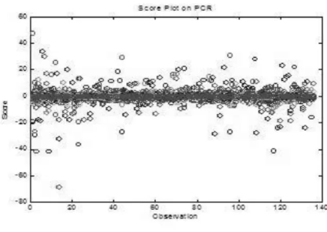
Figure 4 displays the score plot. It explains whether the data follows linear or non-linear. In this experiment, the score plot of PC showed that the data has linear tendency.
[Figure 4] Score Plot on PCR
Figure 5 presents relationship of both eigenvalues and principal components. To determine the number of principal components for construction of a regression model, the eigenvalues versus principal component plot is used from Figure 5. In Figure 5, there is an order changes between 50th and 51st principal component. Thus, 50 principal components will be used to construct a regression model. Those selected principal components explained 96.7475% of total information.
[Figure 5] Plot of Eigenvalues vs. Principal Component
3.4 Partial Least Squares Regression
For the PLSR, two-stage approach will be used.
In the first stage, the data will be scaled like the PCR procedure. After then, training set will be used to find a proper PLSR model continuously in second stage. In that stage, linear or non-linear PLSR will be determined based on the training set. After determination of a model, the test set will be inputted in the model to estimate the responses. The estimated values are compared to the original values in responses using MSE. In Figure 6, the score plot of latent factors in PLSR shows that the data shows linear tendency which is same as PCR.
[Figure 6] Score Plot on PLSR
Figure 7 showed the mean square error versus latent factor graph. From the Figure 7, the number of latent factors will be determined for an appropriate PLSR model. Within the experiment, 12 latent variables are used.
Figure 7: Plot of Mean Square Error vs. Latent Factor
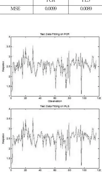
Figure 8 displays the fitting plot of both original and predicted responses with test set on both PCR and PLSR. Table 1 showed that all models' prediction performance using mean square error.
From the Table 1, PCR prediction error is higher than PLSR prediction error. As shown in Figure 8 and Table 1, PLSR is a best prediction model in this experiment. For the experiments, MATLAB software is implemented to use PCR and PLSR for analysis.
In this study, those methods found appropriate models which can be used for new dataset. When the new data (NIR spectra) of diesel fuels is collected, the viscosity level will be predicted through spectra.
<Table 1> Mean Square Error Comparison for Regression, PCR and PLS
PCR PLS
MSE 0.0099 0.0089
[Figure 8] Original vs. Predicted Responses Plot with Test Set on PCR and PLSR (Green: Original, Red:
Predicted)
4. Conclusion
From the section 3, two models (PCR and PLSR) can be used to construct a prediction model for the NIRs data and can be used any data with linear tendency. For the model construction, data scaling will be an important step to avoid the ill-conditioned problem. Also, linearity check with score plots is one of the common steps to decide whether the linear model or non-linear model is used.
To deal with ill-conditioned problem, PCR only removes the collinearity for input space with PCA.
On the contrary, PLSR considers collinearity of both input and output space.
Also determination of both principal components in PCR and latent factors in PLSR is one of important ways to find a proper regression model. Depend on the number of principal components and latent factors, the mean square error will be increased or decreased.
From the experimental results, PLSR gave more proper fitting model for NIRs fuel data. Moreover, the prediction model of PCR is comparable to the PLSR in the used fuel data. Maybe the reason of the finding is that the correlations of both independent variables and response are not higher than 0.7. That is, most of samples are less significantly correlated to the response. But, PLSR can show much better performance than PCR in different applications if dataset are correlated to their responses.
Acknowledgement.
5. References
[1] Dunia R, Qin SJ, Edgar TF, Mcavoy TJ (1996),
“Sensor fault identification and reconstruction using principal component analysis”, Proc. of IFAC Congress'96, pp. 259-264, San Francisco, June 30-July 5
[2] Furtado P, Madeira H (1999), “Analysis of accuracy of data reduction techniques”, First International Conference, DaWaK’99, Florence, Italy, Springer-Verlag, pp. 377-388
[3] Geldi P, Kowalski B (1986), “Partial Least Squares Regression: A Tutorial”, Analytica
Chemica Acta Vol. 185, pp. 1-17
[4] Hines JW, Gribok AV, Attieh I, Uhrig RE (2000),
“Regularization methods for inferential sensing in nuclear power plants”, Fuzzy Systems and Soft Computing in Nuclear Engineering, Chapter 13, Ed. Da Ruan, Springer Verlag
[5] Hoskuldsson A (1988), “PLS Regression Met hods”, Journal of Chemometrics, Vol. 2, pp.
211-228
[6] Sánchez-Franco MJ, Roldán JL (2005), “Web acceptance and usage model: A comparison between goal-directed and experiential web users”, Internet Research, Emerald Group Publishing Limited, Vol. 15, Issue 1, pp. 21-48 [7] Valle-Cervantes S, Li W, Qin SJ (1999), “Selecti
on of the number of principal components: A new criterion with compression to existing meth ods”, I&EC Research, Vol. 38, pp. 4389-4401 [8] Westerhuis JA, De Jong S, Smilde AK (2001),
“Direct orthogonal signal correction”, Chemomet rics and Intelligent Laboratary Systems, Vol. 56, pp. 13-25
[9] Wold H (1966), “Non-linear estimation by iterative least squares procedures”, In: David, F.
(Ed.), Research Papers in Statistics, Wiley, NY [10] Wold H (1985), “Partial least squares”, in Kotz, S.,
Johnson, N.L. (Eds), Encyclopedia of Statistical Sciences, Wiley, New York, NY, Vol. 6, pp. 581-91
저 자 소 개
백 승 현
명지대학교 산업공학과에서 학사학위 를 취득하였고 동일전공으로 미국 조 지아공대에서 석사학위와 미국 테네 시 대학에서 박사학위를 취득하였다.
현재 한양대학교 ERICA 경상대학 경 영학부에서 조교수로 재직중이다. 관 심분야는 데이터마이닝, 품질경영, SCM(공급사슬관리), 생산운용관리, CRM(고객관계관리), 금융공학등이다.
주소: 안산시 상록구 한양대학로 55, 한양대학교 경상대학 경영학부