Numerical Study of the Radiation Potential of a Ship Using the 3D Time-Domain Forward-Speed Free-Surface Green Function and a Second-Order BEM

DOI: 10.3744/SNAK.2008.45.3.258

3 차원 시간영역 전진속도 자유표면 Green 함수와 2 차 경계요소법을 사용한 선체의 방사포텐셜 수치계산

홍 도 천

^†*

, 홍 사 영

^**

충 남 대 학 교 첨 단 수 송 체 연 구 소

^*

한 국 해 양 연 구 원 해 양 시 스 템 안 전 연 구 소

^{* *}

Numerical Study of the Radiation Potential of a Ship Using the 3D Time- Domain Forward-Speed Free-Surface Green Function and a Second-

Order BEM

Do-Chun Hong

^†*

and Sa-Young Hong

^**

Center for Advanced Transportation Vehicles, Chungnam National University

^*

Maritime and Ocean Engineering Research Institute, KORDI

^**

Abstract

The radiation potential of a ship advancing in waves is studied using the 3D time- domain forward-speed free-surface Green function and the Green integral equation.

Numerical solutions are obtained by making use of the 2nd order BEM(Boundary Element Method) which make it possible to take account of the line integral along the waterline in a rigorous manner. The 6 degree of freedom motion memory functions of a hemisphere and the Wigley seakeeping model obtained by direct integration of the time-domain 3D potentials over the wetted surface are presented for various Froude numbers.

※Keywords: Three-Dimensional Time-Domain Forward-Speed Free-Surface Green Function (

3DTFFG

: 3 차원 시간영역 전진속도 자유표면 그린함수), Green integral equation(Green 적분방정 식), Time-domain radiation potential(시간영역 방사파 포텐셜), Radiation m

emory function(운동 이력함수),

2nd order BEM(Boundary Element Method) (2 차경계요소법)

1. INTRODUCTION

A damaged ship advancing in waves suffers

접수일: 2008 년 2 월 15 일, 승인일: 2008 년 5 월 30 일 g교신저자: [email protected], 042-868-7588

varying sinkage, trim and heel due to the flooded compartments. Therefore, it is difficult to analyze the ship motion and wave-loads by using the frequency-domain method (Hong and Hong 2005). A surface-piercing floating body in an arbitrary motion can be analyzed by using the

transient free-surface Green function presented by Stoker (1957). He has also proved the uniqueness of unsteady motions in unbounded domains when surface-piercing obstacles are present, by making use of the free-surface Green function. In the frequency domain, the three-dimensional forward-speed free-surface Green function has been presented by Brard (1948) under integral form, where it has been shown that the behavior of far-field waves is distinct according as the Brard number

Bn

, the product of the Froude number

Fn

and the non- dimensional encounter frequency of the ship with regular incident waves, is greater or smaller than 1/4 known as the critical Brard number. The application of the three dimensional frequency- domain forward-speed Green function to the radiation potential boundary value problem has been attempted by Chang (1977) using a source integral equation. The frequency-domain three- dimensional forward-speed free-surface Green function in the frequency domain approximated by using the complex exponential integral has been presented by Guevel et al. (1979). Some numerical results using the frequency-domain forward-speed free-surface Green function have been presented (Inglis and Price 1981, Maury et al. 2003). Liapis and Beck (1985) have presented the Green integral equation for the radiation problem of a ship advancing with a constant forward-speed using the three- dimensional time-domain forward-speed free- surface Green function (3DTFFG) approximated by series obtained by using the principle of stationary phase. King et al. (1988) have shown the added mass and wave-damping coefficients obtained by using the Fourier transforms of the time-domain numerical results. The above two methods are fully linear and presented in the moving coordinate system fixed in the mean

position of the ship advancing with zero or constant speed of unidirectional velocity. Lin and Yue (1990) have presented a three-dimensional time domain approach formulated in an earth- fixed coordinate system in order to predict the large-amplitude arbitrary motions and wave loads of a ship in a seaway. The body boundary condition is satisfied on the instantaneous wetted surface while the free surface condition is linearized. Bingham et al. (1993) have presented the memory functions as well as the impulse response functions of ships using 3DTFFG approximated by Newman (1992). All the above mentioned methods make use of the free- surface Green function which satisfies the linearized free-surface condition and the constant panel method are employed to obtain numerical solutions. In the present paper, the Neumann-Kelvin linearization is adopted. The radiation potential of ships advancing with a constant speed in waves are calculated using 3DTFFG approximated by Newman (1992). The linear potential problem is solved by using the Green integral equation discretized according to a second-order boundary element method. The Green integral equation at each time-step is solved following the time-stepping procedure presented by Beck and Liapis (1987).

2. FORMULATION

A three-dimensional surface-piercing body of arbitrary shape undergoes arbitrary six-degree- of-freedom motion in the presence of incident waves in a water of infinite depth, the fluid motions can be described by a velocity potential as follows, assuming that the fluid is incompressible, the flow is irrotational and the capillarity is negligible:

( , )

P t

_I( , )

P t

_P( , )

P t

Φ = Φ + Φ (1)

where Φ denotes the incident wave potential, _I Φ the disturbance potential due to the body P

expressed in an earth-fixed cartesian coordinate system ( , , )

x y z . The disturbance potential at a

point

P x y z at a time

( , , )

t

in the fluid region

R(t)

bounded by the mean free surface

F(t)

and the boundary at infinity

S _∞

, can be found using the transient free-surface Green function associated with a source located at a point

Q

( , , )

ξ η ζ

, of a certain disturbance introduced at the time

τ

(Stoker 1957). The transient free-surface Green function

G G

= ( , , ; : , , ; )

ξ η ζ τ x y z t

satisfies the following initial and boundary conditions:

0 0

G G in z for t

t τ

∂ = = = =

∂ (2)

2

2

0 0

G G

g in z

t z

∂ + ∂ = =

∂ ∂

(3)

,

G

,

G

0

G G and at S for t

t t

_∞

τ

∂ ∇ ∇∂ → >

∂ ∂ (4)

The Green function

G has been found as

follows;

( , , )

0 ^S

G P Q t

−

τ

=

G

+

G

(5)

0

( , ) 1/ ( , ) 1/ ( , )

1

G P Q

=

r P Q

−

r P Q

(6)

0

( )

0

( , , ) 2 [1 cos ( )]

( )

S k z

G P Q t gk t

e

^ζ

J k R dk

τ

^∞

τ

+

− =

∫

− − (7)

where

2 2 2

( , ) ( ) ( ) ( )

r P Q

=

x

−

ξ

+

y

−

η

+

z

−

ζ

(8)

2 2 2

1

( , ) ( ) ( ) ( )

r P Q

=

x

−

ξ

+

y

−

η

+

z

+

ζ

(9)

2 2

( ) ( )

R

=

x

−

ξ

+

y

−

η

(10)

and

g

the gravitational acceleration and

J the ₀

Bessel function of order 0.

When the incident wave is absent, the disturbance potential is identical to the radiation potential Φ_R . The initial and boundary

conditions for Φ_R are the same as the conditions given by Eqs. (2)-(4). In addition, Φ satisfies the body boundary condition on R

the wetted surface of the body

S(t)

.

( ) t ⋅ ∇Φ

_R

( , ) M t = ( ) t ⋅ ( , ), M t M on S t ( )

n n V

(11)

where

n

( )

t

is the unit vector normal to

S(t)

pointing out of the fluid region

R(t)

and

V

( , )

M t

the velocity of

S(t)

. Applying the Green theorem to Φ and G in _R

R(t)

, the following Green integral equation can be found after some arrangements using the transport theorem as well as the boundary conditions (Lin and Yue 1990).

0 0

( )

0 ( )

( )

( , )

2 ( , ) [ ( , ) ]

( , )

{ [ ( , ) ]

1 ( , )

[ ( , ) ] ( ) }

R R R

S t t S

S R R

S t

S R S

R

G Q t

P t Q t G dS

n n

G Q

d Q G dS

n n

Q G Q G dL

g

τ τ

ττ τ

τ

π

τ τ τ

τ τ

τ

Γ

∂ ∂Φ

Φ + Φ −

∂ ∂

∂ ∂Φ

= Φ −

∂ ∂

+ Φ − ∂Φ ⋅

∂

∫∫

∫ ∫∫

∫ ^{V N}

(12)

where Γ( )

t

is the waterline of the body and

N the unit normal to

Γ( )

t

on the free surface

F(t)

pointing out of the fluid region

R(t)

. Here, assuming that the body advances with a constant speed U in the positive x-direction accompanying small amplitude six-degree-of- freedom motion, the potential can be expressed in a moving coordinate system ( , , )

x y z attached

to the mean position of the body with the origin in the waterplane of the body and the

z

-axis vertically upwards, as follows.

6 1

( , ) _W( ) _k( , )

k

P t U x P P t

=

Φ = − + Φ +

∑

Φ ⁽¹³⁾

where −

U x

is the free-stream potential, Φ _W the steady disturbance potential due to the constant forward motion of the body and

( 1,2,,,6)

k

k

Φ = the radiation potentials due to the six-degree-of-freedom motion. We will adopt the Neumann-Kelvin linearization which assumes that each disturbance potential, steady or unsteady, as well as the amplitude of the six- degree-of-freedom motion has a magnitude of order

ε

, a quantity as small as the linear wave slope, for example, while the free-stream potential has a magnitude of order 1. By making use of the perturbation analysis, the disturbance potentials and the motions of the body can be developed in powers of

ε

. In the present linearized problem, all terms smaller than the term of order

ε

are neglected. Then the linearized body boundary condition for the unsteady potential Φ_k(

k

=1,2,,,6) can be expressed as follows in the moving coordinate system.

, 1,2,,,6

k

n x

k k

m x on S k

k k

n

∂Φ = ⋅ + =

∂ (14)

where

1 2 3 4 5 6

( , , ),

n n n

( , , )

n n n

= × =

n r n

(15)

3 2

(0, 0, 0, 0,

Un

,

Un

)

= −

m

(16)

and

x

_k ,(

k

=1,2,,,6) denotes the displacement of the six rigid-body modes of motion from its mean position and the overdot the time derivative.

The integral equation for the unsteady potential Φ can be written as follows k

0 0

0

1

( , )

2 ( , ) [ ( , ) ]

( , )

{ [ ( , ) ]

( , )

1 [ ( , )( ) (

( , )

) ] }, 1,2,,,6

k k k

B t S

S k k

B

S S k

k

k S

Q t

P t Q t G G dS

n n

G Q

d Q G dS

n n

G Q

Q G U

g

U Q G U n dL k

τ τ

ττ τ

τ

π

τ τ τ

τ τ

ξ τ

τ ξ

Γ

∂Φ

Φ + Φ ∂ −

∂ ∂

∂ ∂Φ

= Φ −

∂ ∂

∂ ∂Φ

− Φ − −

∂ ∂

− ∂Φ =

∂

∫∫

∫ ∫∫

∫

(17)

where

n

,

S and

Γ denote ( )

n t

,

S(t )

and Γ( )

t

at their mean positions respectively. The Green function

G expressed in the body fixed

coordinate system is as follows.

( , , )

0 ^S

G P Q t

−

τ

=

G

+

G

(18)

0

( , ) 1/ ( , ) 1/ ( , )

1

G P Q

=

r P Q

−

r P Q

(19)

0

( )

0

( , , ) 2 [1 cos ( )]

( )

S k z

G P Q t gk t

e

^ζ

J k R dk

τ

^∞

τ

+

− =

∫

− − (20)

where

2 2 2

( , ) ( ) ( ) ( )

r P Q

=

x

−

ξ

+

y

−

η

+

z

−

ζ

(21)

2 2 2

1

( , ) ( ) ( ) ( )

r P Q

=

x

−

ξ

+

y

−

η

+

z

+

ζ

(22)

2 2

( ( ) ) ( )

R

=

x U t

+ − −

τ ξ

+

y

−

η

(23)

Introducing nondimensional variables

s and υ

as follows;

/ ' ( ), ( ) / '

s

=

g r t

−

τ υ

= − +

z ζ r

(24) with

2 2 2

' [ ( ) ] ( ) ( )

r

=

x U t

+ − −

τ ξ

+

y

−

η

+

z

+

ς

(25) the time derivative of

G ,denoted by ^S G , can ^f

be written as follows:

( , , ) 2 / '3 ( , )

G P Q t

f −

τ

=

g r f s υ

(26)

The function

f s

( , )

υ

for small

s

can be expanded as follows (Lamb 1932):

( )

1 2 1 1

( , ) ( 1) ! ( )

2 1 !

n n

n n

f s s n P

υ ^{+ −} n υ

=

= −

∑

− ⁽²⁷⁾

When

s

is large, it can be written as follows (Newman 1992):

( , )

_{a b}

f s υ

=

f

+

f

(28)

( ) _{2 3}

0

2 2 !

2 ( )

!

a n n

n

f n s P

n ^{− −} υ

=

= −

∑

+ ⁽²⁹⁾

1

2

( / 2 / 4)

4

1 2( ) 2

0 0

2 Re{

2sin

( ) }

sin

s e

i

i i b

n n m n im

mn

n m

f i e

i d e

θ

θ π

θ

θ θ ω

−

−

− +

− + −

= =

= −

∑ ∑

(30)

Where

cos

1

θ

=

⁻ υ

(31)

2

(2 2 2)!

(2 2)!2 !

nm n m

m n

d c

n m

+ −

= −

(32)

2

( 1/ 2)

n

2 !

n

c n

π

n

Γ +

=

(33)

2

2

i s e

i

^θ

ω

=

⁻ (34)

Representing Φ by the following convolution. _k

( )

0^t

( )

k

( )

k

t

φ τk

x t

τ τ

d

Φ = ∫ −

(35) The body boundary condition due to an impulsive body’ s velocity can be obtained as follows

( ) ( ) ( )

k

t n

k

t m H t

k

on S

φ δ

⋅ ∇ = +

n

(36) In this case,

φ

_k can be written as follows

( , ) ( ) ( ) ( ) ( ) ( , )

k

Q t

k

Q t

k

Q H t

k

Q t

φ

=

ϕ δ

+

μ

+

ψ (37)

Then the integral equation (17) can be split into three integral equations as follows by using

G ,

^f the time derivative of

G (Liapis and Beck

^S 1985).

0

0

( , )

2 ( ) ( )

( ) ( , ) , 1,2,,,6

k k

S

k S

G P Q

P Q ds

n n Q G P Q ds k

πϕ

+

ϕ

^∂

∂

= =

∫∫

∫∫

(38)

0

0

( , )

2 ( ) ( )

( ) ( , ) , 5,6

k k

S

k S

G P Q

P Q ds

n m Q G P Q ds k

πμ

+

μ

^∂

∂

= =

∫∫

∫∫

(39)

0

0 2

0

0

( , )

2 ( , ) ( , )

( , , ) ( , )

( , , ) [( ( , )

( , )

( , , ) ]

2 [( ( , ) ( , , )]

( , )

( ) ( , , )

k k

S t f

k S t f

W k

f k

t f

W k

f f

k k

S S

G P Q

P t Q dS

n G P Q t

d Q dS

n

U G P Q t

d d Q

g G P Q t Q

U d d Q G P Q t

g

G Q t

Q dS n G P Q t dS

n

τ

πψ ψ τ

τ ψ τ τ

τ η ψ τ τ

ξ

ψ τ

τ ξ

τ η ψ τ τ

ϕ

+ ∂

∂

∂ −

+ ∂

∂ −

+ ∂

− − ∂

∂

− −

= − ∂ +

∂

+

∫∫

∫ ∫∫

∫ ∫

∫ ∫

∫∫ ∫∫

0

0

( ) ( , , )

( , , ) ( )

t f

k S t f

k S

d m Q G P Q t dS

G P Q t

d Q dS

n

τ τ

τ μ τ

−

∂ −

− ∂

∫ ∫∫

∫ ∫∫

(40)

3.

DISCRETIZATION

OF INTEGRAL EQUATION

In this paper, the integral equations are discretized spatially by using a second-order boundary element method (SOBEM). It is a modified version of the second-order boundary element method (HOBEM) developed by Hong and Choi (1995). In HOBEM, the collocation points are located at the boundary nodes of the second-order element while they are inside the boundary in SOBEM. The position vector of the l

^th

point on the i

^th

element can be written as follows:

8 1

l m m( ),l

i i i i

m

x x N ϖ ϖ ν

_ν

σ

=

=

∑

=

^e

+

^e

^σ

uur uur uur uur

(41)

where ( , )

ν σ

denote a local orthogonal curvilinear coordinates of a eight-node Serendipity second-order quadrilateral boundary element and

N

_i^m the quadratic interpolation functions. A six-node second-order triangular boundary element has also been used in SOBEM.

The potential at the l

^th

point on the i

^th

element can be written as follows:

8 1

( )_i^l _i^m _i^m( )_i^l

m

x N

ϕ ϕ ϖ

=

=

∑

uur uur

(42)

Where

ϕ

_i^m denotes the unknown potential at the m

^th

node of the i

^th

element. For example, the integral equations (38) discretized by using SOBEM can be written as follows:

,

, 8

1

8 0

1 1

8 0

1 1

2 ( )

( ) ( , )

( ) ( , ) 1,2,,, ; 1,2,,, ; 1,2,,,

n j

n j

m m l

i i i

m

Nb m m l l

j j j i j

j m dS

Nb m m l l

j j j i j

j m dS

N

N G x x dS

n N G x x dS

for i Nd l Nc j Nb

π ϕ ϖ

ϕ ϖ

ϖ

=

= =

= =

+

=

= = =

∑

∑∑ ∫∫

∑∑ ∫∫

uur

uur uur uur

uur uur uur

(43)

The integral equations (38) and (39) can be solved by using the constant panel method. But Eq. (40) cannot be solved completely by that method since they have unknown spatial derivatives of potentials along the waterline. By using SOBEM, the unknown derivatives can be represented by a linear combination of the unknown potentials and their given normal derivatives as follows:

8 , 1 1

, , , , 8

, , , , ,

, , , 1

,

,

m m

m

m m

m n

N

N

n n n

ν

ξ ν ν ν

η σ σ σ σ

ξ η ζ

ζ

ψ

ψ ξ η ζ

ψ ξ η ζ ψ

ψ ψ

− =

=

⎡ ⎤

⎢ ⎥

⎢ ⎥

⎢ ⎥

⎡ ⎤ ⎡ ⎤ ⎢ ⎥

⎢ ⎥ ⎢= ⎥ ⎢ ⎥

⎢ ⎥ ⎢ ⎥ ⎢ ⎥

⎢ ⎥ ⎢⎣ ⎥ ⎢⎦ ⎥

⎢ ⎥

⎣ ⎦ ⎢ ⎥

⎢ ⎥

⎢ ⎥

⎣ ⎦

∑

∑

⁽⁴⁴⁾

The SOBEM makes it possible to avoid implying the body boundary condition and the free surface condition at the same point on the waterline nodes. The Eq. (40) discretized by using SOBEM with the aid of Eq. (44) yield overdetermined linear systems for unknown node values. The numerical integration in time has been carried by using the temporal discretization presented by Beck and Liapis (1987).

4. NUMERICAL RESULTS AND DISCUSSIONS

The equations of motion of a ship advancing in waves can be written as follows:

6 1

0

[( ) ( ) ( )

( ) ( ) ( ) ( )

( ), 1,2,,,6

jk jk k jk k

k

t

jk jk k jk k

j

M a x t b x t

C c x t d K t x X t j

τ τ τ

=

+ + +

+ + −

= =

Σ

∫

⁽⁴⁵⁾

Where the coefficients on the left-hand side are as shown by Liapis and Beck(1985). The coefficients

C

_jk denote the well-known hydrostatic restoring coefficients and

M

_jk the ship’ s inertia matrix. In particular, the radiation memory functions can be obtained as follows:

,

1

( ) ( , ) ( , )

( , ) , ( )

j k k t j k j

S S

k l j l

W

K t Q t n dS Q t m dS

dl Q t U n U U

ρ ψ ρ ψ

ρ ψ

= −

− = − ×

∫∫ ∫∫

∫ ^{e l n}

⁽⁴⁶⁾

The

X t

_j( ),(

j

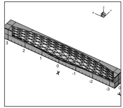
=1,2,,,6) on the right-hand side of Eq.(45) are the six components of the exciting forces and moments due to the diffraction potential which will be presented in the near future.

Numerical tests have been done for a hemisphere and the well known Wigley seakeeping model as shown in Figs.1 and 2

respectively for various Froude numbers. Figs.

3-4 show surge-surge and heave-heave memory functions of the hemisphere. It should be noted that small scale fluctuations persist indefinitely at zero forward speed as shown in Fig. 5. These fluctuations may be due to the numerical errors caused by the spatio-temporal discretization of the time-domain integral equations. In Figs. 6-7, the wave damping coefficients at zero forward speed, calculated by using the improved Green integral equation (IGIE ) which is free of the irregular frequencies (Hong 1987) and the same coefficients calculated from the memory functions by using the Fourier transforms, have been compared with each other. As shown in these figures, the wave damping coefficients via Fourier transform agree quite well with the frequency-domain coefficients but small fluctuations of the former coefficients are seen in the neighborhood of the irregular frequencies which can be found in the solution of the source integral equation. Since the uniqueness of the present problem has already been proven by Stoker (1957) by making use of the transient free-surface Green function as mentioned earlier, the fluctuations must be due to relaxation of the initial conditions caused by the spatio-temporal discretization of the time-domain integral equation and the truncation of the memory functions at

t g a =35 where

/

a

denotes the radius of the hemisphere. The wetted surface of the hemisphere is discretized by 224 six- or eight-node second-order boundary elements and a non-dimensional time-step Δ =

t

0.05

a g

/ has been used.

The memory functions at nonzero forward speed present slowly decaying oscillations with critical period

t _c

which can be obtained by using the critical Brard number of 1/4 as follows:

/ 2 2 /1/ 4, / 2

t c g a

=

π Fn Fn U

=

ag

(47) In Fig. 3, it can be seen that the greater the forward speed the longer the critical period. The large-time oscillation of the memory function at nonzero forward speed can be fitted to a curve of the following form (Bingham et al. 1994):

0 1 2

( ) [ cos( ) sin( )]/

, 2 /

j k c c

c c

K t a a t a t t

t

ω ω

ω π

+ +

= (48)

-3 -2 -1 Y0 1 2 3

-3 -2 -1 0

Z

-2 0

2

X Y Z

X

Fig. 1 Second-order panel representation of hemisphere

0

Y

-3 -2 -1 0 1 2 3

X

Z

X Y

Fig. 2 Second-order panel representation of Wigley model

t (g/L)

^1/2 K11/(ρVg/L)

0 5 10

-0.200.20.40.6

Fn=0 Fn=0.025 Fn=0.05

Fig. 3 Surge-surge memory function of hemisphere

t (g/L)

^1/2 K33/(ρVg/L)

0 5 10

-0.100.10.2 Fn=0

Fn=0.025 Fn=0.05

Fig. 4 Heave-heave memory function of hemisphere

t (g/L)

^1/2 K11/(ρVg/L)

0 10 20 30 40 50

-0.200.20.40.6

Fn=0 Fn=0.025 Fn=0.05

Fig. 5 Large-time behavior of surge-surge memory function of hemisphere

ω²

a/g

B11/ρVω

0 1 2 3 4 5 6 7 8 9 10

00.10.20.30.40.50.6

SOBEM (time-domain) IGIE (frequency-domain)

First irregular freq. (Source integral eq.) Second irregular freq.(Source integral eq.)

Fig. 6 Surge-surge damping coefficients of hemisphere at Fn=0

ω²

a/g

B33/ρVω

0 1 2 3 4 5 6 7 8 9 10

00.10.20.30.40.5

SOBEM (time-domain) IGIE (frequency-domain)

First irregular freq. (Source integral eq.) Second irregular freq.(Source integral eq.)

Fig. 7 Heave-heave damping coefficients of hemisphere at Fn=0

t (g/L)

^1/2 K11/(ρVg/L)

0 2 4

-0.1 0 0.1 0.2 0.3

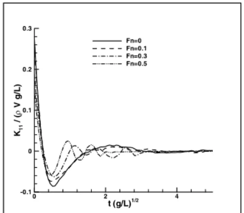
Fn=0 Fn=0.1 Fn=0.3 Fn=0.5

Fig. 8 Surge-surge memory function of Wigley model

t (g/L)

^1/2 K22/(ρVg/L)

0 1 2 3 4 5

-5 0 5 10 15 20

Fn=0 Fn=0.1 Fn=0.3 Fn=0.5

Fig. 9 Sway-sway memory function of Wigley model

t (g/L)

^1/2 K33/(ρVg/L)

0 1 2 3 4 5

-1 0 1 2 3 4

Fn=0 Fn=0.1 Fn=0.3 Fn=0.5

Fig. 10 Heave-heave memory function of Wigley model

t (g/L)

^1/2 K44/(ρVL2g/L)

0 1 2 3 4 5

-0.00200.0020.004 Fn=0

Fn=0.1 Fn=0.3 Fn=0.5

Fig. 11 Roll-roll memory function of Wigley model

t (g/L)

^1/2 K55/(ρVL2g/L)

0 2 4 6

-0.1-0.0500.050.10.15

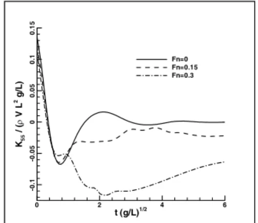
Fn=0 Fn=0.15 Fn=0.3

Fig. 12 Pitch-pitch memory function of Wigley model

t (g/L)

^1/2 K66/(ρVL2g/L)

0 1 2 3 4 5

-0.5 0 0.5 1 1.5

Fn=0 Fn=0.1 Fn=0.3 Fn=0.5

Fig. 13 Yaw-yaw memory function of Wigley model

t (g/L)

^1/2 K55/(ρVL2g/L)

0 5 10 15 20 25 30 35 40 45

-0.1-0.0500.050.10.15

Fn=0 Fn=0.15 Fn=0.3

Fig. 14 Large-time behavior of pitch-pitch memory function of Wigley model

In a two-dimensional study for a submerged body advancing in waves, the added mass and wave damping coefficients have been shown to be finite and continuous but their derivatives are discontinuous at the critical Brard number (Hong 1988). If the nature of the two-dimensional study is similar to the present three-dimensional study, the Fourier transforms should present slowly decaying oscillations with critical period

t _c

. Figs.8-13 show memory functions for the six modes of the Wigley seakeeping model. The wetted surface is discretized by 150 eight- node second-order boundary elements and a non-dimensional time-step Δ =

t

0.075

L g

/ has been used. The pitch-pitch memory functions at

Fn

=0.15 and 0.3 show slowly decaying oscillations with critical period

t _c

and they tend to nonzero constants as shown in Figs.14. Here, the constants have been evaluated by using Eq.(48) and subtracted off and added to the restoring coefficient

c in

_jk the equations of motion (45) as proposed by Bingham et al. (1994).

5. CONCLUSIONS

The radiation potential of a ship advancing in waves is calculated in the time-domain using the three-dimensional time-domain forward-speed free-surface Green function and the Green integral equation on the basis of the Neumann- Kelvin linear wave hypothesis.

The integral equation for the potential is discretized according to a second-order boundary element method (SOBEM) where the collocation points are located inside the panel.

The SOBEM makes it possible to take account of the line integral along the waterline in a rigorous manner.

The wave damping coefficients of a

hemisphere at

Fn

=0, calculated from the memory functions by using Fourier transform, have been shown to agree quite well with the frequency-domain coefficients.

The numerical results of the memory functions related to the six-degree-of-freedom motions of a hemisphere and the Wigley seakeeping model have successfully been obtained for various Froude numbers.

Acknowledgments

The present work is a part of the research programs on the development of simulation technology for dynamic stability of ships, granted by the Korea Ministry of Knowledge Economy.

REFERENCES

• Beck, R.F. and Liapis, S.J., 1987, “Transient Motion of Floating Bodies at Zero Forward Speed,” J. of Ship Research, Vol. 31-3, pp.

164-176.

• Beck, R.F. and Reed, A.M., 2001, “Modern Computational Methods for Ships in Seaway,”

Trans. SNAME, Vol. 109, pp. 1-48.

• Bingham, H.B., Korsmeyer, F.T., Newman, J.N.

and Osborne, G.E., 1993, “The Simulations of Ship Motions,” Proceedings, 6th Int. Conf. on Numerical Ship Hydrodynamics, pp. 561-579

• Bingham, H.B., Korsmeyer, F.T. and Newman, J.N., 1994, “ Prediction of the Seakeeping Characteristics of Ships,” Proceedings 20

^th

Symp. on Naval Hydrodynamics, pp. 27-46

• Brard, R., 1947, “ Introduction to the Theoretical Study on the Pitch Motion of an Advancing Ship (in French),” Bulletin of L’ ASSOCIATION TECHNIQUE MARITIME ET AERONAUTIQUE, Vol. 47, Paris, 1948.

• Chang, M.S., 1977, “Computation of Three- Dimensional Ship Motion with Forward Speed,” Proceedings 2

^nd

Int. Conf. on Num.

Ship Hydrodynamics, University. Of California, Berkely

• Guevel, P., Bougis, J. and Hong, D.C., 1979,

“ Formulation of the Problem of the Oscillations of the Floating Bodies Advancing with Constant Forward Speed and Excited by Incident Waves (in French),” Summary of the 4

^th

Congrès Français de Mécanique, Nancy, France, pp. 324-325

• Hong, D.C., 1987, “On the Improved Green Integral Equation Applied to The Water-Wave Radiation-Diffraction Problem,” Journal of the Society of Naval Architecture of Korea, Vol.

24, No.1, pp. 1-8.

• Hong, D.C., 1988, “Unsteady Wave Generation by an Oscillating Cylinder Advancing under the Free Surface,” Journal of the Society of Naval Architecture of Korea, Vol. 25, No. 2, pp. 11- 18.

• Hong, D.C. and Hong, S.Y., 2005, “Waveload Analysis for Heeled Barges with Flooded Compartiments(in Korean),” Journal of the Society of Naval Architecture of Korea, Vol. 42, No. 4, pp. 379-387.

• Hong, S.Y. and Choi, H.S., 1995, “Analysis of Steady and Unsteady Flow around a Ship using a Higher-Order Boundary Element Method (in Korean),” Journal of the Society of Naval Architecture of Korea, Vol. 32, No. 1, pp. 42-57.

• Inglis R.B. and Price, W.G., 1982, “A Three Dimensional Ship Motion Theory, Comparison between Theoretical Predictions and Experimental Data of the Hydrodynamic Coefficients with Forward Speed,” Trans.

RINA Vol. 124, pp. 141-157.

• King, B., Beck, R.F. and Magee, A. 1988, Seakeeping Calculations with Forward Speed using Time-Domain Analysis, Proceedings, 17th Symposium on Naval Hydrodynamics, The Hague, Netherlands, pp. 577-596.

• Lamb, H., 1932 “Hydrodynamics,” 6

^th

Edition Cambridge Univ. Press, p. 431

• Liapis, S. and Beck, R.F. 1985, Seakeeping Computations using Time-Domain Analysis, Proceedings, 4th International Conference on Numerical Ship Hydrodynamics, pp. 34-56.

• Lin, W.M. and Yue, D.K.P., 1990, “Numerical Solutions for Large-Amplitude Ship Motions in the Time Domain,” Proceedings 18

^th

Symp.

on Naval Hydrodynamics, pp. 41-66.

• Maury, C., Delhommeau, G., Ba, M., Boin, J.P.

and Guilbaud, M., 2003, “Comparison between Numerical Computations and Experiments for Seakeeping on Ship Models with forward Speed,” Journal of Ship Research, Vol. 47, No. 4, pp. 347-364.

• Newman, J.N., 1992, “Approximation of Green Functions,” Wave Asymptotics, Proceedings Fritz Ursell Meeting, Cambridge Univ. Press, pp. 107-135.

• Stoker, J.J., 1957 “Water Waves,”

Interscience Publishers, New York, pp. 187- 196.