영상 복원을 위한 통합 베이즈 티코노프 정규화 방법
류재흥*
A Unified Bayesian Tikhonov Regularization Method for Image Restoration
Jae-Hung Yoo
*요 약
본 논문은 영상 복원 문제에 대한 정규화 모수를 찾는 새로운 방법을 제시한다. 사전 정보가 없으면 티코노프 (Tikhonov) 정규화 모수를 선택하기 위한 일반화된 교차 검증법이나 L자형 곡선 검정 등의 별도의 최적화 함수 가 필요하다. 본 논문에서는 티코노프 정규화에 대한 통합된 베이즈 해석을 소개하고 영상 복원 문제에 적용한 다. 티코노프 정규화 모수와 베이즈 하이퍼 모수들의 관계를 정립하고 최대 사후 확률과 근거 프레임워크를 사 용한 정규화 모수를 구하는 공식을 제시한다. 실험결과는 제안하는 방법의 효능을 보여준다.
ABSTRACT
This paper suggests a new method of finding regularization parameter for image restoration problems. If the prior information is not available, separate optimization functions for Tikhonov regularization parameter are suggested in the literature such as generalized cross validation and L-curve criterion. In this paper, unified Bayesian interpretation of Tikhonov regularization is introduced and applied to the image restoration problems. The relationship between Tikhonov regularization parameter and Bayesian hyper-parameters is established. Update formular for the regularization parameter using both maximum a posteriori(: MAP) and evidence frameworks is suggested. Experimental results show the effectiveness of the proposed method.
키워드
Bayesian Interpretation, Evidence Framework, Tikhonov Regularization, Image Restoration 베이즈 해석, 근거 프레임워크, 티코노프 정규화, 영상 복원
* 교신저자: 전남대학교 컴퓨터공학과 ㆍ접 수 일 : 2016. 11. 01 ㆍ수정완료일 : 2016. 11. 13 ㆍ게재확정일 : 2016. 11. 24
ㆍReceived : Nov. 01, 2016, Revised : Nov. 13, 2016, Accepted : Nov. 24, 2016 ㆍCorresponding Author : Jae-Hung Yoo
Dept. of Computer Engineering, Chonnam Nat. Univ.
Email : [email protected]
Ⅰ. Introduction
Image restoration is the process to recover an original image from distorted one by using an appropriate degradation model[1]. Image restoration is an example of inversion problems in the ill-posed systems[2,3]. In the linear degradation model, we assume that a given input image is blurred by a Point Spread Function(: PSF) and
further distorted by a Gaussian noise . This can be written in the form
⋆ (1)
where symbol⋆denotes convolution.
In the Fourier transform, we have
. (2)
http://dx.doi.org/10.13067/JKIECS.2016.11.11.1129
In the inverse filtering, we have
. (3)
This formula shows that if is zero or very small in the high frequency region and is still not vanished in the corresponding region, the second term is amplified. Thus we need a remedy solving ill-posed inverse problem.
Wiener filter requires priori information such as power spectrums of original image and noise. If the noise level is known a priori, Morozov's Discrepancy Principle(: MDP) can be applied for the determination of regularization parameter in the constrained least squares image restoration.
Otherwise separate optimization functions such as Generalized Cross Validation(: GCV) function and L-curve criterion are suggested as alternative methods in the literature[4-7].
In this paper, unified Bayesian interpretation of Tikhonov regularization is suggested and applied to the image restoration problems. In section II, square residual and smoothing term in the frequency domain are introduced to solve for Tikhonov regularization parameter. In section III and IV, Bayesian update of Tikhonov regularization parameter is introduced and applied to the image restoration problems. The relationship between Tikhonov regularization parameter and Bayesian hyperparameters is established. Update formular for the regularization parameter using both Maximum A Posteriori(: MAP) and evidence frameworks is suggested. In section V, experimental results show the effectiveness of the proposed method followed by the conclusion and reference sections.
Ⅱ. Regularization Parameter Selection in the Frequency Domain
In the Tikhonov regularization for an ill-posed problem , we seek a limiting vector
to fit data in least squares sense with penalty term for large normed solution in the cost function as
∥ ∥
∥ ∥
. (4)
Regularized estimation vector is defined as
. (5)
Here, and are the block circulant matrices of a PSF and a smoothing operator respectively.
Smoothing functional usually given by the Laplacian operator. is the Tikhonov regularization parameter. and
are the column vectors stacking columns of a degraded image and a recovered image
respectively. Both and
matrices have the dimension, MN by MN. That is, m = n = MN with image dimension M by N.
In the frequency domain, block circulant matrices
and are diagonalized. We denote them and
respectively. Let and be the column vectors of the Fourier transform of and respectively.
Regularized estimation vector is defined as
, (6)
where superscript denotes the Hermitian or conjugate transpose.
Square residual is defined as
∥
∥
. (7)
Here, and are the diagonal elements of the
matrices and respectively.
is the element of column vector stacking columns of 2D Fourier transform of the degraded image .
Smoothing term is defined as
∥
∥
. (8)
Ⅲ. Unified Bayesian Interpretation of Tikhonov Regularization
MAP estimator maximizes the posterior pdf
which can be expressed using Bayes' law[8] as following
, (9)
×
. (10)
Assume that both error and original image are Gaussian random vectors, we have
∥ ∥
, (11)
∥ ∥
. (12) By taking the negative log for the Bayes' law, we have the MAP interpretation of Tikhonov regularization as
. (13)
We can interpret the parameter as a global scalar proportionality measure analogous to the parametric Wiener filter with setting to the identity matrix.
In the evidence framework[9], we have fixed-point iteration known as the MacKay update
≡
, (14)
≡
(15)
or
, (16)
. (17)
In these equations, and are unknown hyper-parameters
,
. (18)
and
are regularization and cost terms respectively
∥ ∥
, (19)
∥∥
(20)
and is the number of effective parameters
. (21)
Here,
and
denote singular value of
and
respectively.
Then we combine the MAP and the evidence
frameworks into the unified Bayesian update
formular for the Tikhonov regularization
parameter as a fixed point iteration method.
(22)
with
. (23)
Now we have the unified Bayesian interpretation of Tikhonov regularization.
Ⅳ. A New Image Restoration Method using Unified Bayesian Regularization
We have the Bayesian update formular for the Tikhonov regularization parameter in the frequency domain using equation (7) and (8) as
∥ ∥
∥∥
, (24)
≡
(25)
with
. (26)
Here, we see that the number of effective parameters is equal to the sum of filter factors[10].
After calculating using the fixed point iteration, we obtain as following
(27)
where superscript denotes the Hermitian or
conjugate transpose.
Reshaping the column vector into 2D matrix to obtain , we finally get the estimation of original image by taking inverse 2D FFT.
Ⅴ. Experimental Results
We report the experiments with the new image restoration method proposed in the previous two sections. Figure 1 shows the satellite image data from the USAF Phillips Laboratory, Laser and Imaging Directorate, Kirtland AFB, NM[11].
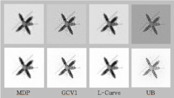
We compare the unified Bayesian(: UB) method with the conventional techniques MDP, GCV, L-curve and Wiener filter. Results are depicted in the figures 2 , 3 and 4. First row shows the restored image data having negative pixel components and the second row further processed by using projection with non-negativity constraint.
Visual inspection shows that MDP and L-curve results in an over smoothed estimation with Laplacian smoother and GCV depicts under smoothing with identity matrix.
Fig. 1 Satellite image data.
Fig. 2 Restored images with Wiener filter as benchmark.
Fig. 3 Restored images with Laplacian smoother.
Fig. 4 Restored images with identity smoother.
The new UB method shows comparable results with conventional methods using smoothing operator. However, the UB filter depicts under smoothing with identity matrix that is more severe compared to the GCV method.
Image restoration performance is measured by the figure-of-merit functions such as relative error (RE), signal to noise ratio (SNR), peak SNR (PSNR) and improvement of SNR (ISNR)[7,12-14].
Table 1 and 2 show the image restoration performance with remarking value of regularization parameter . Results of Wiener filter is included for comparison benchmark. Here, we report only the restored image data projected with non-negativity constraint. We have the equivalent results as visual inspection on the restored images.
Measure
Method RE↓ SNR↑ PSNR ISNR Remark
MDP 0.3803 8.397 22.03 5.356 8.29e-2 GCV 0.3449 9.247 22.87 6.206 4.45e-3 L-curve 0.4509 6.917 20.55 3.876 1.00e-0 UB 0.3489 9.146 22.77 6.106 7.91e-3 Wiener 0.3243 9.781 23.41 6.740 N/A
Table 1. Performance Results using Laplacian smoother with Wiener filter as benchmark.
Measure
Method RE↓ SNR↑ PSNR ISNR Remark
MDP 0.3648 8.758 22.39 5.717 4.75e-4 GCV 0.3575 8.935 22.56 5.895 9.80e-5 L-curve 0.3623 8.818 22.45 5.777 4.38e-4 UB 0.5694 4.891 18.52 1.850 1.72e-5
Table 2. Performance Results with identity smoothing operator.
Ⅵ. Conclusions
In this paper, unified Bayesian interpretation of
Tikhonov regularization is suggested and applied to
the image restoration problems. The relationship
between Tikhonov regularization parameter and
Bayesian hyper-parameters is established. Update
formular for the regularization parameter using both
maximum a posteriori and evidence frameworks is
suggested. Fixed point iteration can be applied for
the regularization parameter. Experimental results
show the comparable performance of the unified
Bayesian method.
References
[1] R. Gonzalez and R. Woods, Digital Image Processing. Reading, MA: Addison-Wesley, 1992.
[2] H. Engl, M. Hanke, and A. Neubauer, Regularization of Inverse Problems. Dordrecht:
Kluwer Academic Publishers, 1996.
[3] S. Kim, "An image denoising algorithm for the mobile phone cameras," J. of the Korea Institute of Electronic Communication Sciences, vol. 9, no. 5, 2014, pp. 601-608.
[4] G. Golub, M. Heath, and G. Wahba,
"Generalized cross-validation as a method for choosing a good ridge parameter,"
Technometrics, vol. 21, no. 2, 1979, pp. 215-223.
[5] P. Hansen and D. O’Leary, "The use of the L-curve in the regularization of discrete ill-posed problems," Society for Industrial and Applied Mathematics J. on Scientific Computing, vol. 14, no. 6, 1993, pp. 1487-1503.
[6] V. Morozov, Methods for Solving Incorrectly Posed Problems. New York: Springer-Verlag, 1984.
[7] J. Yoo, "Self-Regularization Method for Image Restoration," J. of the Korea Institute of Electronic Communication Sciences, vol. 11, no.
1, 2016, pp. 45-52.
[8] R. Duda and P. Hart, Pattern Classification and Scene Analysis. New York: John Wiley & Sons, 1973.
[9] D. MacKay, "Bayesian interpolation," Neural Computation, vol. 4, no. 3, 1992, pp. 415-445.
[10] P. C. Hansen, Rank-Deficient and Discrete Ill-Posed Problems: Numerical Aspects of Linear Inversion, Philadelphia: Society for Industrial and Applied Mathematics, 1998.
[11] J. Nagy, K. Palmer, and L. Perrone, "Iterative methods for image deblurring: a Matlab object oriented approach," Numerical Algorithms, vol. 36, no. 1, 2004, pp. 73-93.
[12] Y. Kim, "A Study on Fractal Image Coding," J. of the Korea Institute of Electronic Communication Sciences, vol. 7, no. 3, 2012, pp.
559-566.
[13] C. Lee and J. Lee, "Implementation of Image Improvement using MAD Order Statistics for SAR Image in Wavelet Transform
Domain," J. of the Korea Institute of Electronic Communication Sciences, vol. 9, no.
12, 2014, pp. 1381-1388.
[14] S. Park, "Optimal QP Determination Method for Adaptive Intra Frame Encoding," J. of the Korea Institute of Electronic Communication Sciences, vol. 10, no. 9, 2015, pp. 1009-1018
저자 소개(Author)
류재흥(Jae-Hung Yoo)