Solution of Klein Gordon Equation for Some Diatomic Molecules Bull. Korean Chem. Soc. 2014, Vol. 35, No. 12 3443 http://dx.doi.org/10.5012/bkcs.2014.35.12.3443
Solution of Klein Gordon Equation for Some Diatomic Molecules with
New Generalized Morse-like Potential Using SUSYQM
Cecilia N. Isonguyo, Ituen B. Okon, Akpan N. Ikot,†,* and Hassan Hassanabadi‡ Theoretical Physics Group, Department of Physics, University of Uyo-Nigeria
†Theoretical Physics Group, Department of Physics, University of Port Harcourt, Choba, PMB 5323, Port Harcourt-Nigeria *E-mail: [email protected]
‡Department of Basic Sciences, Shahrood Branch, Islamic Azad University, Shahrood, Iran Received April 24, 2014, Accepted August 6, 2014
We present the solution of Klein Gordon equation with new generalized Morse-like potential using SUSYQM formalism. We obtained approximately the energy eigenvalues and the corresponding wave function in a closed form for any arbitrary l state. We computed the numerical results for some selected diatomic molecules. Key Words : New generalized Morse-like potential, Supersymmetric quantum mechanics, Klein Gordon equation
Introduction
In quantum mechanics, the study of exact solutions of relativistic and non-relativistic equation with different potentials plays a significant role in Physics.1-5 The bound state solution of Klein Gordon equation (KGE) is of great important in nuclear and high energy physics.6 Klein Gordon equation is a relativistic wave equation that describes spin-zero particles. It contains of two major objects, the vector potential V(r) and the scalar potential S(r). In D-dimension, the Klein Gordon equation5 is written as
(1) where Enl is the energy and m is rest mass.7,8 However, different authors have adopted several techniques to obtain the exact or approximate solutions of KGE with various potential interactions. These techniques include asymptotic
iteration method (AIM),9 the Nikiforov-Uvarov method
(NU),10 supersymmetric quantum mechanices,11 and others. Amongst the potentials studied with these techniques are the Manning-Rosen Potential,12,13 Hulthen Potential,14,15 Eckart-type Potential,16,17 Wood-Saxon Potential,18,19 Poschl-Teller Potential.20 Many contributions from different authors shows that the analytical solution of KGE are possible only in the
s-wave case (l = 0) while for , it is solved by using
suitable approximation scheme.21,22 The Morse Potential is one of the known potentials model used in describing diatomic molecules. It given as
, (2)
Where De is the dissociation energy, r0 is the equilibrium
internuclear distance and a is a parameter controlling the width of potential well.23 Nevertheless, several authors have done investigations with this potential, Berkdemir investi-gated Pseudospin symmetry in relativistic Morse potential including the spin-orbit coupling,23 Jia et al. studied Equi-valence of the deformed Rosen-Morse Potential energy model and Tietz potential energy model,24 Zarezadeh et al. investigated the solution of the Schrodinger wave equation for a particular form of Morse Potential using Laplace transform,25 Erkol et al. studied the Exact solutions for a Hamiltonian with Morse Potential and Dirac Delta shell interactions.26
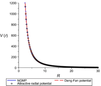
In this work, we introduced a novel potential and call it the New Generalized Morse-like potential (NGMP) model re-cently proposed by Ikot et al.27 having the same behaviours as MP, attractive radial potential and Deng-Fan potential models. It is defined as d2 dr2 --- + Enl2 + V2( ) − 2Er nlV r( ) − m2 − S2( ) − 2mS rr ( ) − D( +2l 1+ ) D 2l 3( + + ) 4r2 --- Ψnl( ) = 0r l 0≠ V r( ) = De⎛⎝e–2a r r(– 0)–e–a r r(–0)⎠⎞ De>0, a 0>
Figure 1. Behavior of potentials for α = 0.01 fm−1, a = 1, b = −2, c = 1, d = −1, De=−0.8 fm−1.
3444 Bull. Korean Chem. Soc. 2014, Vol. 35, No. 12 Cecilia N. Isonguyo et al.
(3) where a, b, c, d, are constant coefficients and the term in the bracket is the Mobius square potential proposed recently (see Fig. 1).
The purpose of our work is to investigate the Solution of Klein Gordon equation for some diatomic molecules with NGMP using Supersymmetry Quantum mechanics.
Klein-Gordon in D-dimension
The Klein-Gordon equation in higher dimension for spheri-cally symmetric potential reads,22-25
(4) Where En,l, m, V(r) and S(r) are the relativistic energy ,rest mass, the repulsive vector potential and the attractive scalar potential respectively and ΔD is defined as
(5) The total wave function in D-dimension is written as,
(6)
The term is the generalization of the centrifugal
term for the higher dimensional space. The eigenvalues of are defined by the relation,
(7)
Where and l represent the hyperspherical
harmonics, the hyperradial wave function and the orbital angular momentum quantum number respectively.
Now substituting ansatz for the
wave function into Eq. (4) yields,
(8)
Solutions of the Radial Klein-Gordon Equation in D-dimension
Now considering equal scalar and vector potentials as the
NGMP, in Eq. (7), we obtain the second order
Schrodinger-like equation For equal scalar and vector potentials = , substituting Eqn. (3) into Eqn. (1), we have
(9)
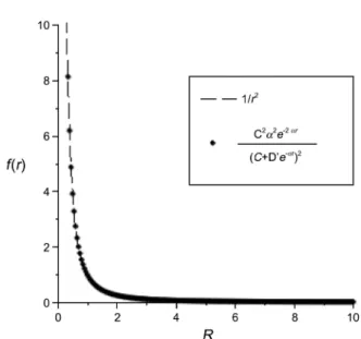
The good approximation for the centrifugal term is given as,28
, (10)
where c = −d, Eq. (10) gives a good approximation for the centrifugal term (see in Fig. (2)). When performing a power
series expansion and setting gives the desired r−2
suggested by Greene and Aldrich.29
Now, Substituting Eq. (10 ) into (9) we have,
= (11) Furthermore, we can rewrite Eq. (11) as follows:
, (12) Where, (13) (14) (15) V r( ) = De 1 a be αr – + c de+ –αr ---⎝ ⎠ ⎛ ⎞2 – ΔD – ψn,l,m(r,ΩD) = E{[ n l,–V r( )]2− m S r[ + ( )]2}ψn,l,m(r,ΩD) ΔD = ∇D2 = 1 rD 1– ---∂ ∂ -- rD 1– ∂r---∂ ⎝ ⎠ ⎛ ⎞ −ΛD2(ΩD) r2 ---ψn,l,m(r, ΩD) = Rn l,( )Yr lm(ΩD) ΛD 2 Ω D ( )/r2 ΛD 2 Ω D ( ) ΛD2(ΩD)Ylm(ΩD) = l l D 2( + – )Ylm(ΩD) Ylm(ΩD), Rn l, Rn l,( ) = rr D 1– ( ) 2 ---– Fn l,( )r d2 dr2 --- + Enl2 + V2( ) − 2Er nlV r( ) − m2 − S2( ) − 2mS rr ( ) − D( +2l 1+ ) D 2l 3( + + ) 4r2 --- Ψnl( ) = 0r S r( ) = V r( ) V r( ) S r( ) d2 dr2 --- + Enl2 − m2 − 2 E( nl+m)De1 a be αr – + c de+ –αr ---⎝ ⎠ ⎛ ⎞2 ⎝ ⎠ ⎛ ⎞ – − D( +2l 1+ ) D 2l 3( + + ) 4r2 --- Ψnl( ) = 0r 1 r2 ---- = α2 ce αr – c de+ –αr ---⎝ ⎠ ⎛ ⎞2 = α 0lim→ 1 r2 ---- α r --- 5 12 ---α2 1 12 ---α3r 1 240 ---α4r2 + + + + ⎝ ⎛ 1 720 ---α5r3 – 1 6045 ---α6r4 – +O r( )5⎠⎞ α 0→ d2ψnl dr2 ---+ 1 1 de–α r c ---+ ⎝ ⎠ ⎛ ⎞ ---2Deb2(Enl+m) c --- α2(D 2l 1+ – ) D 2l 3( + – ) 4 ---– ⎝ ⎠ ⎛ ⎞e–2αr +4Deab E( nl+m)e–α r+2Dea2(Enl+m) ψnl( )r m2–Enl2+ D2 e(Enl+m) [ ]ψnl( )r d2ψnl dr2 ---– + Veff( )ψr nl( ) = E˜ψr nl( )r Veff( ) = Xer 2αr – + Ye–αr + Z 1 de αr – c ---+ ⎝ ⎠ ⎛ ⎞2 ---X = 2Deb 2 Enl+m ( ) c ---– + α 2 D 2l 1+ – ( ) D 2l 3( + – ) 4 ---Y = 4– Deab E( nl+m)
Figure 2. The centrifugal term (1/r2) and its approximation for α = 0.01 fm−1, c = 1, d = −1.
Solution of Klein Gordon Equation for Some Diatomic Molecules Bull. Korean Chem. Soc. 2014, Vol. 35, No. 12 3445
(16) (17) To be able to solve Eq. (12), we have to solve the associated Riccati equation
, (18)
for which we propose a solution of the form
. (19)
Substituting Eq. (19) into Eq. (18), we get
(20)
Solving Eq. (20), we obtain the following three set of parameters
(21)
, (22)
(23)
Now based on Eq. A.2, we can obtain the supersymmetric partner potentials as,
(24)
Therefore, it is shown that and are shape
invariant, satisfying the shape-invariant condition
, (25)
with ρ0= f and ρ1 is a function of ρ0, i.e .
Therefore, . Thus, we can see that the shape
invariance holds via a mapping of the form .
From Eq. (A.5), we have
,
,
·
· (26)
,
The energy eigenvalues can be obtained as follows
, (27)
where,
, (28)
By substituting Eqs. (23) and (28) into Eq. (27), We have
(29)
More explicitly, we obtain the energy equation for the Klein Gordon equation with NGMP as
+ (30) Where , (31) (32) Z = 2– Dea2(Enl+m) E˜nl = Enl2 − m2− 2De(Enl+m) W2( ) W′r +− ( ) = Vr eff( ) − E˜r 0,l W r( ) = fe αr – 1 de αr – c ---+ ⎝ ⎠ ⎛ ⎞ --- + q f2e–2αr 1 de α r – c ---+ ⎝ ⎠ ⎛ ⎞2 --- + q( )2 + 2f qe α r – 1 de αr – c ---+ ⎝ ⎠ ⎛ ⎞2 --- + α fe αr – 1 de α r – c ---+ ⎝ ⎠ ⎛ ⎞2 = Xe 2α r – Ye–αr Z + + 1 de α r – c ---+ ⎝ ⎠ ⎛ ⎞2 --- − E˜0,l E˜0,l = − q( )2 + Z f = dα c ---⎝ ⎠ ⎛ ⎞ ± dα c ---⎝ ⎠ ⎛ ⎞2 + 4 X d2Z c2 --- dY c ---– + ⎝ ⎠ ⎛ ⎞ 2 ---q = f2 – X d 2 Z c2 ---– + ⎝ ⎠ ⎛ ⎞ 2fd c --- ---Veff+( ) = r f f dα c ---+ ⎝ ⎠ ⎛ ⎞e–2αr 1 de αr – c ---+ ⎝ ⎠ ⎛ ⎞2 --- + 2f qe αr – 1 de αr – c ---+ ⎝ ⎠ ⎛ ⎞ --- + q( )2 Veff−( ) = r f f dα c ---– ⎝ ⎠ ⎛ ⎞e–2αr 1 de αr – c ---+ ⎝ ⎠ ⎛ ⎞2 --- + 2f qe αr – 1 de αr – c ---+ ⎝ ⎠ ⎛ ⎞ --- + q( )2 Veff+( )r Veff−( )r V+(r, ρ0) = V−(r, ρ1) + R ρ( )1 ρi = f ρ( ) = ρ0 0 + dα---c ρn = ρ0 + dαn⎝⎛---c ⎠⎞ f→ + dαf c ---⎝ ⎠ ⎛ ⎞ R a( ) = 1 ρ02 – X Zd 2 c2 ---– + 2ρ0d c --- ---⎝ ⎠ ⎜ ⎟ ⎜ ⎟ ⎜ ⎟ ⎛ ⎞2 − ρ12 – X Zd 2 c2 ---– + 2ρ1d c --- ---⎝ ⎠ ⎜ ⎟ ⎜ ⎟ ⎜ ⎟ ⎛ ⎞2 R a( ) = 2 ρ12 – X Zd 2 c2 ---– + 2ρ1d c --- ---⎝ ⎠ ⎜ ⎟ ⎜ ⎟ ⎜ ⎟ ⎛ ⎞2 − ρ22 – X Zd 2 c2 ---– + 2ρ2d c --- ---⎝ ⎠ ⎜ ⎟ ⎜ ⎟ ⎜ ⎟ ⎛ ⎞2 R a( ) = n ρn 12– – X Zd 2 c2 ---– + 2ρn 1– d c --- ---⎝ ⎠ ⎜ ⎟ ⎜ ⎟ ⎜ ⎟ ⎛ ⎞2 − ρn2 – X Zd 2 c2 ---– + 2ρnd c --- ---⎝ ⎠ ⎜ ⎟ ⎜ ⎟ ⎜ ⎟ ⎛ ⎞2
E˜nl = E˜nl− + E˜0,l
E˜nl− = k 1= n
∑
R a( ) = k ρ02 – X Zd 2 c2 ---– + 2ρ0d c --- ---⎝ ⎠ ⎜ ⎟ ⎜ ⎟ ⎜ ⎟ ⎛ ⎞2 − ρn2 – X Zd 2 c2 ---– + 2ρnd c --- ---⎝ ⎠ ⎜ ⎟ ⎜ ⎟ ⎜ ⎟ ⎛ ⎞2 E˜nl = − ρn2 – X Zd 2 c2 ---– + 2ρnd c --- ---⎝ ⎠ ⎜ ⎟ ⎜ ⎟ ⎜ ⎟ ⎛ ⎞2 + Z Enl2 –m2– D2 e(Enl+m) c2 4d2 ---2Deb2(Enl+m) c ---– +α--- 2D2(D 2l 1+ –4) D 2l 3( + – )+ ea2(Enl+m)d2 c2 ---⎝ ⎠ ⎜ ⎟ ⎜ ⎟ ⎜ ⎟ ⎛ ⎞ dα c ---⎝ ⎠ ⎛ ⎞ n σ[ + ] --- 1– + 2Dea2(Enl+m) = 0 ρn = dα c ---⎝ ⎠ ⎛ ⎞ n σ[ + ] σ = 1±1 1 4c2 2Deb2(Enl+m) c ---– +α---2(D 2l 1+ –4) D 2l 3( + – ) 2d2Dea2(Enl+m) c2 ---– 4dDeab E( nl+m) c ---+ ⎝ ⎠ ⎜ ⎟ ⎜ ⎟ ⎜ ⎟ ⎜ ⎟ ⎛ ⎞ d2α2 ---+3446 Bull. Korean Chem. Soc. 2014, Vol. 35, No. 12 Cecilia N. Isonguyo et al.
Furthermore, in order to calculate the radial wave function we used the coordinate transform, s = e−αr in Eq. (12) to get,
, (33) The corresponding radial wave function is obtain from Eq. (33) as follows,
(34)
where Nnl is the normalization constant
In order to test for the accuracy of our work, we use the potential parameters given in Ref. [30] Table 1 to compute the energy eigen values for some diatomic molecules of HF2,
N2, I2, H2 and O2 as shown in Tables 2-16, where we have
chosen =1 in our calculation. Conclusion
In this work, we solve the Klein Gordon Equation for NGMP with proper approximation to the centrifugal term using the SUSQM technique. We obtain explicitly, the bound state energy eigenvalues and the corresponding wave function in a closed form. We employed the Aldrich and Greene approximation scheme29 to deal with centrifugal term in d-dimension. However, one may find the improved approximation scheme in Ref. [31, 32] for comparison. Finally, we computed the energy eigenvalues of our work numerically in order to check the accuracy of our results and our result may find many applications in molecular and chemical physics. As compared to the one reported by Chen et al.33 in D-dimension
Acknowledgments. We authors thanks the referee for his/
her technical comments on our manuscript. And the publi-cation cost of this paper was supported by Korean Chemical Society.
References
1. Yi, L. Z.; Diao, Y. F.; Liu, J. Y.; Jia, C. S. Phys. Lett. 2004, 33, 212.
2. Zang, X. C.; Liu, Q. W.; Jia, C. S.; Wang, L. Z. Phys. Lett. A 2005, 340, 59.
3. Qiang, W. C.; Dong, S. H. EPL 2010, 89, 10003.
4. Serrano, F. A.; Gu, X. Y.; Dong, S. H. J. Math. Phys. 2010, 51, 082103.
5. Lucha, W.; Schoberl, F. F. Int. J. Mod. Phys. A 2002, 17, 2233. 6. Antia, A. D.; Ikot, A. N.; Akpan, I. O.; Owoga, O. A. Indian J.
Phys. 2013, 87, 155.
7. Alhaidari, A. D.; Bahlouli, H.; Hasan, A. L. Lett. Phys. A 2006, 349, 87.
8. Ikot, A. N. Chin. Phys. Lett. 2012, 29, 6. 9. Baraket, T. Int. J. Mod. Phys. A 2006, 21, 4127. 10. Nikiforov, A. F., 1988.
11. Setare, M. R.; Nazari, Z. Acta Polonica B 2009, 40(10), 2809. 12. Taskin, F. Int. J. Theor. Phys. 2009, 48, 1142.
13. Manning, M. F.; Rosen, N. Phys. Rev. 1933, 44, 953. 14. Saad, N. Phys. Scr. 2007, 76, 623.
15. Ikot, A. N.; Akpabio, L. E.; Uwah, E. J. EJTP 2011, 8(25), 225. 16. Jia, C. S.; Gao, P.; Peng, X. L. J. Phys. A. Math. Gen. 2006, 39,
7737.
17. Guo, J. Y.; Sheng, Z. Q. Phys. Lett. A 2005, 388, 90. 18. Ikot, A. N.; Akpan, I. O. Chin. Phys. Lett. 2012, 29, 090302. 19. Alhaidar, A. D. Found. Phys. 2010, 40, 10885.
20. Poshl, G.; Teller, E. Z. Phys. 1933, 83, 623.
21. Arda, A.; Server, R.; Tezcan, C. Phys. Scr. 2009, 79, 5006. 22. Arda, A.; Server, R. Int. J. Theor. Phys. 2009, 48, 945. 23. Berkdemir, C. Nucl. Phys. A 2006, 770, 32.
24. Jia, C. S.; Chen, T.; Yi, L. Z.; Lin, S. R. J. Math. Chem. 2013, 51, 2165.
25. Zarezadeh, M.; Tavassoly, M. K. Chin. Phys. C 2013, 37, 4. 26. Erkol, H.; Demialp, E. Molecular Phys. 2009, 107, 19.
27. Ikot, A. N.; Maghsoodi, E.; Zarrinkamar, S.; Hassanabadi, H. J. Theor. Phys. 2013, 7, 53.
28. Yazarloo, B. H.; Hassanabadi, H.; Rahimovi, S. Euro. Phys. J. Plus 2012, 127, 51.
29. Greene, R. L.; Aldrich, C. Phys. Rev. A 1976, 14, 2363.
30. Kunc, J. A.; Gordillo-Vazquez, F. J. J. Phys. Chem. A 1997, 101, 1595.
31. Jia, C. S.; Chen, T.; Cui, L. G. Phys. Lett. A 2009, 373, 1621. 32. Jia, C. S.; Diao, Y. F.; Yi, L. Z.; Chen, T. Int. J. Mod. Phys. A
2009, 24, 4519.
33. Chen, X. Y.; Chen, T.; Jia, C. S. Euro. J. Phys. Plus 2014, 129, 75. 34. Ikot, A. N.; Maghsoodi, E.; Ibanga, E. J.; Zarrinkamar, S.;
Hassanabadi, H. Chin. Phys. B 2013, 22, 120302.
35. Cooper, F.; Khare, A.; Sukhatme, U. Phys. Rep. 1995, 251, 267. d2ψnl ds2 --- + 1 d c ---s + ⎝ ⎠ ⎛ ⎞ s 1 d c ---s + ⎝ ⎠ ⎛ ⎞ ---dψnl ds --- + 1 s2 1 d c ---s + ⎝ ⎠ ⎛ ⎞2 ---X α2 --- E˜nld 2 α2c2 ---– ⎝ ⎠ ⎛ ⎞ – s2+ 2E˜nld cα2 --- Y α2 ---– ⎝ ⎠ ⎛ ⎞s − Z α2 --- E˜nl α2 ---– ⎝ ⎠ ⎛ ⎞ ψnl( )=0s Rnl( ) = Nr nl(e–α r) Z α2 --- E˜nl α2 ---– 1 d c ---e–αr + ⎝ ⎠ ⎛ ⎞ d – 2c --- d2 4c2 --- X α2 --- Yd cα2 ---– Zd2 c2α2 ---+ + −d c --- Z α2 --- E˜nl α2 ---– ⎝ ⎠ ⎜ ⎟ ⎛ ⎞ – Pn 2 Z α2 --- E˜nl α2 ---– , 2 d2 4c2 --- X α2 --- Yd cα2 ---– Zd2 c2α2 ---+ + ⎝ ⎠ ⎜ ⎟ ⎛ ⎞ 1 2d c ---e– rα + ⎝ ⎠ ⎛ ⎞ h