Atmos. Meas. Tech., 8, 4025–4041, 2015 www.atmos-meas-tech.net/8/4025/2015/ doi:10.5194/amt-8-4025-2015
© Author(s) 2015. CC Attribution 3.0 License.
Uncertainties of satellite-derived surface skin temperatures in the
polar oceans: MODIS, AIRS/AMSU, and AIRS only
H.-J. Kang1, J.-M. Yoo2, M.-J. Jeong3, and Y.-I. Won4
1Department of Atmospheric Science and Engineering, Ewha Womans University, Seoul 120-750, Republic of Korea 2Department of Science Education, Ewha Womans University, Seoul 120-750, Republic of Korea
3Department of Atmospheric and Environmental Sciences, Gangneung-Wonju National University,
Gangneung 210-702, Republic of Korea
4Wyle ST&E, NASA/GSFC, Maryland, USA Correspondence to: J.-M. Yoo (yjm@ewha.ac.kr)
Received: 11 February 2015 – Published in Atmos. Meas. Tech. Discuss.: 4 May 2015 Revised: 17 July 2015 – Accepted: 9 September 2015 – Published: 2 October 2015
Abstract. Uncertainties in the satellite-derived surface skin temperature (SST) data in the polar oceans during two pe-riods (16–24 April and 15–23 September) 2003–2014 were investigated and the three data sets were intercompared as follows: MODerate Resolution Imaging Spectroradiometer Ice Surface Temperature (MODIS IST), the SST of the At-mospheric Infrared Sounder/Advanced Microwave Sounding Unit-A (AIRS/AMSU), and AIRS only. The AIRS only al-gorithm was developed in preparation for the degradation of the AMSU-A. MODIS IST was systematically warmer up to 1.65 K at the sea ice boundary and colder down to
−2.04 K in the polar sea ice regions of both the Arctic and Antarctic than that of the AIRS/AMSU. This difference in the results could have been caused by the surface classi-fication method. The spatial correlation coefficient of the AIRS only to the AIRS/AMSU (0.992–0.999) method was greater than that of the MODIS IST to the AIRS/AMSU (0.968–0.994). The SST of the AIRS only compared to that of the AIRS/AMSU had a bias of 0.168 K with a RMSE of 0.590 K over the Northern Hemisphere high latitudes and a bias of −0.109 K with a RMSE of 0.852 K over the Southern Hemisphere high latitudes. There was a system-atic disagreement between the AIRS retrievals at the bound-ary of the sea ice, because the AIRS only algorithm uti-lized a less accurate GCM forecast over the seasonally vary-ing frozen oceans than the microwave data. The three data sets (MODIS, AIRS/AMSU and AIRS only) showed signifi-cant warming rates (2.3 ± 1.7 ∼ 2.8 ± 1.9 K decade−1) in the northern high regions (70–80◦N) as expected from the
ice-albedo feedback. The systematic temperature disagreement associated with surface type classification had an impact on the resulting temperature trends.
1 Introduction
The satellite observations of the polar oceans have been more challenging than those of non-frozen ocean and land, be-cause it is more difficult to identify clouds over the various surfaces (Tobin et al., 2006). The surface skin temperature (SST) is one of the most important climate variables that is related to the surface energy balance and the thermal state of the atmosphere (Jin et al., 1997). Compared to ground-based observations, satellite-observed SST data play a cru-cial role in climate study and model development by provid-ing uniform resolution data encompassprovid-ing the entire globe. The retrievals of AIRS data over the last decade have a signif-icant contribution to various climate studies and model eval-uations (Aumann et al., 2003; Tian et al., 2013; Yoo et al., 2013). AIRS retrievals have produced atmospheric temper-ature, moisture, and ozone profiles on a global scale by the AIRS method itself or together with other instruments (Liu at al., 2008). A lot of comparisons of the AIRS/AMSU data against data from numerical forecast model analysis fields, radiosondes, lidar, and retrievals from high-altitude aircraft have been used to assess the accuracy of the retrievals (Tobin et al., 2006; Susskind et al., 2014). The AIRS retrieval algo-rithm has been developed and validated gradually with clear
sky and clear/cloudy conditions over a non-frozen ocean and then the non-polar land and polar cases (Tobin et al., 2006).
The AIRS/AMSU has an advantage of measuring the radi-ation penetrating through clouds and polar darkness, and has high spectral resolution and coarse spatial resolution (Dong et al., 2006). However, the AIRS only algorithm using only AIRS observations has been developed due to the degrada-tion of the AMSU-A. Microwave and multispectral radiome-ters were used for global mapping of the sea ice extent and dynamics, while the visible, near-infrared, and infrared sen-sors could obtain details on the ice concentration, snow/ice albedo, thickness, and IST during clear-sky conditions (Hall et al., 2004; Scott et al., 2014). The MODIS on Earth Ob-serving System (EOS) Aqua, used as infrared measurements, was influenced by water and cloud contamination, but had a higher spatial resolution (Dong et al., 2006). In order to re-move the cloud effects in the MODIS IST algorithm, MODIS cloud mask products were used (Hall et al., 2004).
Since AIRS and MODIS were co-located on Aqua, they have often been used to make a synergistic algorithm and they have been compared to each other frequently (Molnar and Susskind, 2005; Li et al., 2012; Liu et al., 2014). Li et al. (2012) compared the atmospheric instability from at a single AIRS field of view (FOV; ∼ 13.5 km at nadir) sound-ing with that of AIRS/AMSU soundsound-ing (∼ 45 km), utilizsound-ing the MODIS cloud information. Molnar and Susskind (2005) validated the accuracy of the AIRS/AMSU cloud products using MODIS cloud analyses, which have a higher spatial resolution than that of AIRS. Knuteson et al. (2006) com-pared the MODIS Collection 4 (C4) with the AIRS Ver-sion 3 (V3) on the land surface temperature (LST) for the eastern half of the US, showing that the monthly differ-ences were approximately 3 K. Lee et al. (2013) investigated the characteristics of the differences between the MODIS land surface skin temperature/sea surface temperature and the AIRS/AMSU surface skin temperature across the globe, and found that the MODIS C5 product was systematically lower by 1.7 K than the AIRS/AMSU V5 product over land in the 50◦N–50◦S regions, but it was higher by 0.5 K than the AIRS/AMSU product over ocean. Particularly in the sea ice regions, the MODIS annual averages were larger than the AIRS/AMSU values, due to the differential errors in ice/snow emissivity between the retrieval methods (or chan-nels) for the two data products. The differences between the MODIS and AIRS methods were reduced when the MODIS IST and AIRS/AMSU surface skin temperatures were com-pared for 9 days. The possible reasons for this include the lo-cal time of satellite observation difference between them due to the different swath width in the high latitude regions, and the emissivity difference between microwave and infrared channels, but more comparison studies are necessary for a longer period to pin down the reasons of such skin tempera-ture discrepancies between MODIS and AIRS/AMSU.
The primary purpose of this study was to investigate a rel-ative degree of agreement (or disagreement) among
differ-ent SST data sets using the MODIS IST C5, the SST of the AIRS/AMSU, and AIRS only V6. The second purpose of this paper was to analyze the temperature trend differences affected by the temperature differences among different data products. The data sets used in this study were described in Sect. 2. In Sect. 3, we compared the MODIS and AIRS only data with the AIRS/AMSU values. We also analyzed the temperature trends from the three satellite-based data sets in Sect. 4, and in the conclusion we summarized our study.
2 Data and methods
The Aqua satellite carrying the AIRS, AMSU and MODIS instruments was launched on 4 May 2002 with the Earth’s Radiant Energy System (CERES), Humidity Sounder for Brazil (HSB) and the Advanced Microwave Scanning Radiometer-EOS (AMSR-E). It has far exceeded its designed life span of 6 years and has a chance of operating into the 2020’s (http://aqua.nasa.gov/). The Aqua satellite orbits the earth every 98.8 min with an equatorial crossing time go-ing north (ascendgo-ing) at 1:30 p.m. local time (daytime) and going south (descending) at 1:30 a.m. (nighttime) in a sun-synchronous, near polar orbit with an inclination of 98.2◦and an operational altitude of 705 km (Tian et al., 2013).
As shown in Table 1, we used the data sets of MODIS IST (e.g., Hall and Riggs, 2015) and SSTs of AIRS/AMSU and AIRS only over the Northern Hemisphere during 16–24 April and over the Southern Hemisphere on 15–23 Septem-ber from 2003 to 2014 in order to avoid the polar night when the visible channels of the MODIS did not operate (Hall et al., 2004). The sea surface temperature observed from in-frared channels of satellites indicates the values at the skin of sea water, in contrast with the sea surface temperature mea-sured from buoys, of which values represent the temperature of bulk water near the sea surfaces. The infrared sea SST was measured at depths of approximately 10 µm within the oceanic skin layer (∼ 500 µm) at the water side of the air– sea interface where the conductive and diffusive heat trans-fer processes dominated (Emery et al., 2001; Donlon et al., 2002; Liou, 2002).
As an imaging spectroradiometer, the MODIS with 36 bands has retrieved various physical parameters such as aerosol optical thickness, land and water surface tempera-ture, leaf area index, and snow cover, etc. (Barnes et al., 1998; Hall and Riggs, 2007). MODIS produced the “sea ice by reflectance” and “IST” in order to identify sea ice (Riggs et al., 1999). The “sea ice by reflectance” was determined by the normalized difference snow index (NDSI), and the re-flectance of Band 1 (0.645 µm) and Band 2 (0.858 µm). The NDSI was calculated using Band 4 (0.555 µm) and Band 7 (2.130 µm). IST is used as another method for identifying sea ice. The IST derived from the “split-window method” in Eq. (1), where bands 31 and 32 are centered at approximately 11 and 12 µm, respectively. The method was applied in order
H.-J. Kang et al.: Uncertainties of satellite-derived surface skin temperatures in the polar oceans 4027
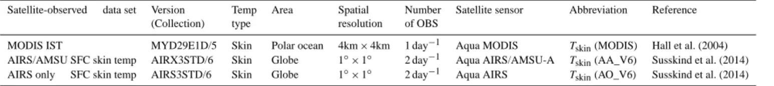
Table 1. The information on the satellite-observed surface skin temperature (Tskin)Level 3 (L3) data used in this study. Three data sets of Tskin were compared over the Northern Hemisphere during 16–24 April 2003–2014, and over the Southern Hemisphere during 15–
23 September 2003–2014. The abbreviations used in this table are as follows: temp (temperature), IST (ice surface skin temperature), OBS (observation), and SFC (surface).
Satellite-observed data set Version Temp Area Spatial Number Satellite sensor Abbreviation Reference (Collection) type resolution of OBS
MODIS IST MYD29E1D/5 Skin Polar ocean 4km × 4km 1 day−1 Aqua MODIS Tskin(MODIS) Hall et al. (2004)
AIRS/AMSU SFC skin temp AIRX3STD/6 Skin Globe 1◦×1◦ 2 day−1 Aqua AIRS/AMSU-A Tskin(AA_V6) Susskind et al. (2014)
AIRS only SFC skin temp AIRS3STD/6 Skin Globe 1◦×1◦ 2 day−1 Aqua AIRS Tskin(AO_V6) Susskind et al. (2014)
to identify the ice when the IST was less than 271.5 K. The cutoff temperature between water and ice (271.5 K) may vary depending on the region and season. The IST is calculated as follows:
IST = a + bT11+c(T11−T12)
+d[(T11−T12)(sec(θ ) − 1)], (1)
where T11is the brightness temperature (K) in 11 µm, T12is
the brightness temperature (K) in 12 µm, and θ is the scan angle from nadir. The difference between the T11 and the
skin temperature from the LOWTRAN can be less than 3 K for a skin temperature between 230 and 260 K (Key et al., 1997). Since the value of T11 itself was a good estimate,
co-efficients a–d were defined for the following temperature ranges: T11< 240 K, 240 K ≤ T11≤260 K, and 260 K < T11
(Riggs et al., 2006). The IST algorithm was only applied to the polar ocean pixels that were determined to be clear by the MODIS cloud mask using visible reflectance (Hall et al., 2004). The surface in the IST algorithm was assumed to be snow (Key et al., 1997). MODIS ISTs were provided as daily polar fields with a 4 km × 4 km resolution.
The AIRS spectrometer is a high spectral resolution trometer with 2378 channels in the thermal infrared spec-trum and 4 bands in the visible specspec-trum (Won, 2008). The AIRS and AMSU were coupled in order to play a role as an advanced sounding system under clear and cloudy condi-tions (Aumann et al., 2003). The AIRS/AMSU algorithm is independent of the GCM, except for the use of GCM surface pressure to determine the bottom boundary conditions (Mol-nar and Susskind, 2005). V6 is the most current retrieval al-gorithm since the launch of AIRS instrument, and detailed descriptions are given in Olsen (2013b). The primary prod-ucts from AIRS suite include the atmospheric temperature-humidity profiles, ozone profiles, sea/land surface skin tem-perature (SST), and cloud related parameters such as the out-going longwave radiation (OLR) (Susskind et al., 2011). In the AIRS/AMSU algorithm, the surface classification was conducted using the brightness temperature difference in 23 GHz (AMSU ch1) and 50 GHz (AMSU ch3). The dif-ference (brightness temperature at 23 GHz minus brightness temperature at 50 GHz) had a negative value on the sea ice and a positive value on the water (Grody et al., 1999; Hewi-son and English, 1999). Also, the brightness temperature
dif-ference between 23 GHz (AMSU ch1) and 31 GHz (AMSU ch2) could distinguish the age of the sea ice (Kongoli et al., 2008). The accuracy of AIRS/AMSU SST can be affected by surface misclassification, which is caused by the surface emissivity changes, the pixel mixed with the various surface types, and the ice pixel pooled with water.
After the surface type classification from the AMSU re-trieval, the initial state for atmospheric and surface param-eters, cloud parameters and OLR was generated using the Neural Network methodology (Susskind et al., 2011, 2014). The methodology was used to approximate some functions between the input and output vectors by training (Gardner and Dorling, 1998). Next, the initial clear column radiances were generated, which were based on the initial state and the observed infrared radiances. The surface and atmospheric variables, including the surface skin temperature, were re-trieved by updating the cloud-cleared infrared radiance, iter-atively. The cloud properties and outgoing longwave radia-tion were then retrieved, followed by the error estimates and quality control. In the AIRS only V6, shortwave window re-gion 3.76–4.0 µm was used in order to derive the surface skin temperature and surface spectral emissivity (ε).
AMSU channels 4–5 had not been available since 2007 and 2010, respectively, due to radiometric noise. In prepa-ration for the degradation of the other AMSU channels, the AIRS only algorithm was developed excluding the AMSU observations. The algorithm was similar to that of AIRS/AMSU, but it did not use the AMSU-A observations in any step of the physical retrieval process and the quality con-trol methodology. The AIRS only algorithm has utilized the forecast surface temperature from the NOAA Global Fore-cast System (GFS) in order to determine whether the oceanic surface is highly likely to be liquid or frozen, instead of AMSU observations (Olsen, 2013a; Susskind et al., 2014).
AIRS/AMSU L2 product (AIRX2RET) is based on 3 × 3 AIRS FOVs coexisting within a single AMSU footprint, and the horizontal resolution of AIRS and AMSU is approxi-mately 13.5 and 45 km, respectively (Aumann et al., 2003; Zheng et al., 2015). The L2 data set of AIRS only is provided on 3 × 3 AIRS FOVs (∼ 45 km) like that of AIRS/AMSU. The two L3 products of the AIRS/AMSU and AIRS only data sets used in this study have also been analyzed under
the same spatial resolution of a 1◦×1◦(∼ 100 km × 100 km)
grid (Table 1).
We calculated the climatology and anomaly values from the yearly 9-day mean temperatures in a 1◦×1◦grid for the 12-year period of Aqua satellite observations in order to esti-mate the temperature anomaly trends. The trends of MODIS IST were derived only when the number of yearly data was at least 10 out of 12 entire years at each grid point. The trends of the AIRS/AMSU and AIRS only were derived only when the number of yearly data sets was 12, covering the entire years of the analysis at each grid. The bootstrap method (Wilks, 1995) was used to calculate at a 95 % confidence interval. In the method, 10 000 linear temperature trends were generated by random sampling, allowing repetition of 10 000 yearly anomaly temperature data sets. Then, we estimated the 95 % confidence interval of 10 000 temperature trends.
3 Comparison of the satellite-derived surface skin temperatures: IST vs. SST
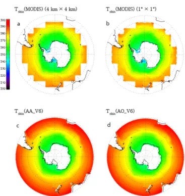
Figure 1a shows the spatial coverage and the averaged value of the MODIS IST over the Southern Hemisphere during 15– 23 September 2003–2014. In order to solve the spatial res-olution mismatches, the original resres-olution of the MODIS data with a 4 km × 4 km grid (Fig. 1a) was re-gridded to a 1◦×1◦grid in the case of MODIS data present over 50 % (Fig. 1b). A grid spacing of 1◦corresponds to approximately 111 km on the equator, and it becomes reduced poleward. In the zonal averaged SST analysis, this 50 % criterion was used. During the same period, the spatial distributions of the climatological Tskin(AA_V6) and Tskin(AO_V6) were also
shown in Fig. 1c–d, respectively. As expected, the MODIS and AIRS showed the spatial distribution of the climatolog-ical SST, warmer at the lower latitudes than the higher lati-tudes. The SST distributions over the Northern Hemisphere during 16–24 April 2003–2014 have been shown in Kang and Yoo (2015).
Figure 2a displays the number of years when both Tskin
(MODIS) and Tskin(AA_V6) are available at each grid point
over the Southern Hemisphere. The number near 60◦S was smaller than that of the other regions because the MODIS IST algorithm only produced its data in the cloud-free pix-els. Similar distributions by the clouds were shown in Fig. 2b and 2d for the same reason. The reduced number of obser-vations near 60◦S had a spatial distribution similar to that
of the frontal cloud bands that were likely associated with the mid-/high-latitude depressions encircling the Antarctica (e.g., Jakob, 1999; Comiso and Stock, 2001; Lachlan-Cope, 2010; Boucher et al., 2013). Figure 2c shows the number of years when both Tskin (AO_V6) and Tskin (AA_V6) were
available at each grid. Most of the grids had both Tskin
(AO_V6) and Tskin (AA_V6) for a period of more than
10 years.
Figure 1. (a) 12-year composite skin temperatures (K) of the
MODIS IST over the Southern Hemisphere during 15–23 Septem-ber 2003–2014. The original MODIS data (MYD29E1D) have a 4 km × 4 km spatial resolution. Their spatial resolution has been re-constructed to 1◦×1◦in (b) in order to compare this data with the AIRS/AMSU data. (c)–(d) is the surface skin temperatures of the AIRS/AMSU and AIRS only over the Southern Hemisphere ocean during 15–23 September 2003–2014, respectively.
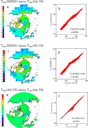
Figure 3a presents the spatial distribution of the tempo-ral difference in a 1◦×1◦ grid between the climatologi-cal Tskin (MODIS) and Tskin (AA_V6) during 16–24 April
2003–2014 over the Northern Hemisphere. In general, Tskin
(MODIS) at 60–70◦N was higher than the Tskin (AA_V6). Tskin(MODIS) was about 3 K higher than the Tskin(AA_V6)
on the Hudson Bay and near Greenland, whereas it was about
−2 K lower near the center of the Arctic Ocean. The rela-tionship between the climatological Tskin(MODIS) and Tskin
(AA_V6) was presented in the scatter diagrams (Fig. 3b). The scatter plot revealed a temperature interval which devi-ated from the simple linear line. The discontinuous shape ap-peared at the freezing point (∼ 273 K) and the turning point (∼ 260 K) in terms of Tskin (MODIS), changing the
coef-ficient of the MODIS IST algorithm. In the interval, Tskin
(MODIS) was systematically higher than the Tskin(AA_V6)
in the 260–273 K range of Tskin(MODIS). The slope in the
range was 0.85, lower than the slope for the whole regression line (0.97). There was a better agreement in the 240–260 K range, where the difference between the T11 and the SST in
H.-J. Kang et al.: Uncertainties of satellite-derived surface skin temperatures in the polar oceans 4029
Figure 2. The number of co-located observations of (a) Tskin
(MODIS) and Tskin (AA_V6), (b) Tskin (MODIS) and Tskin (AO_V6), and (c) Tskin (AO_V6) and Tskin (AA_V6) over the
Southern Hemisphere during 15–23 September 2003–2014. (d) Same as in (c) except for three different data sets (Tskin(MODIS), Tskin(AA_V6), and Tskin(AO_V6)).
better agreement in the range greater than 280 K was also shown.
Figure 3c was the same as Fig. 3a except for Tskin
(MODIS) vs. Tskin (AO_V6). The differences between the
two data sets were very similar to those in Fig. 3a. However,
Tskin(MODIS) was more than 4 K higher than Tskin(AO_V6)
in some regions near the Greenland and the Barents Sea. The slope (0.93) in the 260–273 K range of Tskin(MODIS) also
indicated a deviation from the total slope (0.98) in the scatter plot (Fig. 3d), similar to that in Fig. 3b. Figure 3e showed the difference between Tskin(AO_V6) to Tskin(AA_V6).
Over-all, the agreement was much better than the previous two cases (Fig. 3a and c), except for in the Greenland Sea, the Barents Sea, and the Okhotsk Sea. Both Tskin(AO_V6) and Tskin(AA_V6) agreed with each other (r = 0.999) well
ex-cept for near the freezing point.
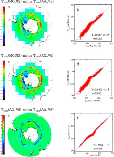
Figure 4 showed discrepancies among the three types of SST data sets over the Southern Hemisphere during 15– 23 September 2003–2014. It has been noted that there was a latitudinal band encircling Antarctica at 60–70◦S, where
Tskin(MODIS) was higher than both the Tskin(AA_V6) and Tskin (AO_V6) (Fig. 4a and c). The circular region
corre-sponded to the sea ice/water boundary which was expected to move seasonally. This implies a systematic difference be-tween Tskin(MODIS) and Tskin(AA_V6) in the sea ice
classi-fication. The corresponding scatter plots also revealed a
dis-Figure 3. The distributions of (a) Tskin (MODIS) minus Tskin
(AA_V6), (c) Tskin(MODIS) minus Tskin(AO_V6), and (e) Tskin
(AO_V6) minus Tskin(AA_V6) over the Northern Hemisphere dur-ing 16–24 April 2003–2014. The scatter plots of (b) Tskin(MODIS)
vs. Tskin(AA_V6), (d) Tskin(MODIS) vs. Tskin(AO_V6), and (f)
Tskin(AO_V6) vs. Tskin(AA_V6).
continuous (i.e., not linear) shape in the 260–273 K range of
Tskin(MODIS) (Fig. 4b and d). The slopes in that range were
0.84–0.94, which were smaller than the slope (0.98) in the whole range. In addition, Tskin(MODIS) showed lower
tem-perature values than Tskin(AA_V6) and Tskin(AO_V6) near
the Antarctic peninsula, in the region from Weddell Sea to Ross Sea (Fig. 4a and c).
The comparison between two types of AIRS data sets also showed the circular pattern around Antarctica where
Tskin(AO_V6) was lower by 1.5–5.6 K than Tskin(AA_V6)
(Fig. 4e). The discrepancy near the sea ice/water boundary was clear, possibly due to the difference in the sea ice de-tection method between the two data sets. The uncertainty of the SST at the sea ice boundary was distinguished from the other regions. Both Tskin(AO_V6) and Tskin(AA_V6) were
re-Figure 4. Same as in Fig. 3 except for the data taken during 15–
23 September 2003–2014, over the Southern Hemisphere.
gions. The scatter pattern of the Tskin (AA_V6) vs. that of
the Tskin (AO_V6) showed that the two data sets generally
agreed with each other, but the disagreement near the freez-ing point again occurred indicatfreez-ing a cold bias of AIRS only with respect to AIRS/AMSU (Fig. 4f).
Figure 5 showed the annual-average spatial distributions for Tskin (MODIS) minus Tskin (AA_V6) in the Southern
Hemisphere from 15–23 September 2003–2014. Although the 9-day composite values were used in each year, Tskin
(MODIS) data did not exist in some areas. It was because the MODIS IST algorithm was valid only for cloud-free pix-els. The systematic positive values at the boundary of the sea ice consistently occurred, while the negative ones occurred on some areas of the sea ice near Antarctica every year.
Figure 6 presented the interannual variation of the spatial distribution of Tskin (AO_V6) minus Tskin(AA_V6) for the
study period. As already seen in Fig. 4e, the values of Tskin
(AO_V6) compared to Tskin(AA_V6) show systematic
neg-ative values encircling Antarctica during the period. In ad-dition, there were positive values over the sea-ice prevailing areas inside the circle, with the location varying from year to
year, which must be related to the difference in the surface type characterization.
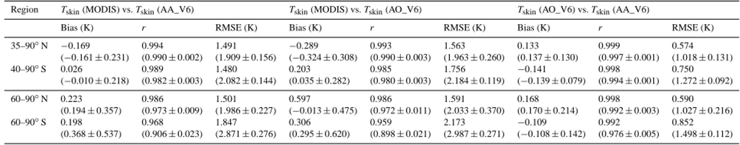
Table 2 showed the statistics of bias, spatial correlation coefficient (r), and root mean square error (RMSE) obtained from the 12-year climatologies of 2003–2014 in order to an-alyze the systematic error among the three types of satellite-observed temperatures quantitatively. This analysis for each hemispheric vernal period has been performed over the two regions (35–90, 60–90◦N) of the Northern Hemisphere dur-ing 16–24 April, and over the regions (40–90, 60–90◦S) of the Southern Hemisphere during 15–23 September. The spatial correlation coefficient between the two satellite data sets was computed in this study as follows. (i) The clima-tological 9-day composite data of SSTs during 2003–2014 were computed in a 1◦×1◦ grid of the two data sets, re-spectively. (ii) We computed the spatial correlation coeffi-cient between the two data sets, using their climatological values in a 1◦×1◦ grid within a given latitude band. The
values in parentheses indicated the average obtained from the statistics for each year and their corresponding standard de-viations. Based on the climatology values, the SST of the AIRS retrievals were comparable with respect to the Tskin
(MODIS) (r = 0.959–0.994). Tskin (MODIS) tended to
sys-tematically exceed the AIRS retrievals over the polar oceans (bias = 0.198–0.597 K). Hall et al. (2004) reported the accu-racy of Tskin(MODIS) with the bias values of 1.2–1.3 K near
the South Pole and the Arctic Ocean. The RMSE of 1.847 K for Tskin (MODIS) vs. the Tskin(AA_V6) over 60–90◦S in
our study was slightly higher than that in the study of Hall et al. (2004).
From the intercomparison of the three data sets, the bias (−0.109–0.597) and RMSE (0.590–2.173) over the high latitude belt (60–90◦N and ◦S) tended to be larger, and
the correlation coefficients (r = 0.959–0.986) was smaller than those over 35–90◦N and 40–90◦S among the three comparisons (Table 2). This result indicated that there was more disagreement over the high latitudes than over other regions. The spatial correlation coefficient (0.992–0.999) between Tskin (AO_V6) and Tskin (AA_V6) was greater
than those (0.968–0.994) between Tskin (MODIS) and Tskin
(AA_V6). In the high latitudes Tskin (AO_V6) with respect
to Tskin (AA_V6) had a positive bias of 0.168 K with a
RMSE of 0.590 K in the Northern Hemisphere, but a bias of −0.109 K with a RMSE of 0.852 K in the Southern Hemi-sphere. The high correlations (r = 0.998–0.999) between the AIRS/AMSU and AIRS only (i.e., AIRS retrievals) over the 35–90◦N and 40–90◦S areas showed that the AIRS only
can be a good alternative for the AIRS/AMSU, except for at the region of the sea ice boundary (r = 0.992 over the 60– 90◦S). The disagreement between Tskin (AA_V6) and Tskin
(AO_V6) at the region where the sea ice and water mixed ap-peared, because the AIRS only used less accurate GCM fore-cast data for surface classification over the potentially frozen oceans.
H.-J. Kang et al.: Uncertainties of satellite-derived surface skin temperatures in the polar oceans 4031
Figure 5. Annual-average spatial distributions of the Tskin (MODIS) minus Tskin (AA_V6) over the Southern Hemisphere during 15–
23 September.
Figure 7 presents the zonal mean temperature difference among the three satellite-observed data sets in a 1◦×1◦ grid over the Northern Hemisphere during 16–24 April 2003–2014 and over the Southern Hemisphere during 15– 23 September 2003–2014. The red, blue and green lines rep-resent the zonally averaged annual values of Tskin(MODIS)
minus Tskin(AA_V6), Tskin(MODIS) minus Tskin(AO_V6),
and Tskin(AO_V6) minus Tskin(AA_V6), respectively. The
climatological annual values have been calculated from the interannually varying yearly data, shown in Fig. 8. The black dashed line, the difference between the original MODIS IST data (4 km × 4 km) and converted Tskin (MODIS) (1◦×1◦)
indicated the possible error from the conversion of spatial
resolution. The differences by the conversion over both hemi-spheres were within 0.3 and 0.5 K, respectively. The original
Tskin (MODIS), converted Tskin (MODIS), Tskin (AA_V6),
and Tskin(AO_V6) were chosen under the same condition in
space and time, and each grid (1◦×1◦) of a degree latitudinal band.
It is hard to see in Fig. 3a the systematic difference due to the sea ice detection over the Northern Hemisphere be-cause of the continental distribution. However, Fig. 7 clearly showed that the difference among the Tskin (MODIS), Tskin
(AA_V6), and Tskin (AO_V6) existed over the Northern
Hemisphere. Tskin(MODIS) was warmer than Tskin(AA_V6)
in 56–81◦N and 54–69◦S, while cooler than T
Table 2. Statistical comparisons of the climatological 9-day composite data during 2003–2014 over both hemispheres; Tskin(MODIS) vs.
Tskin(AA_V6), Tskin(MODIS) vs. Tskin(AO_V6), and Tskin(AO_V6) vs. Tskin(AA_V6). The values in this table were calculated based
on the 12-year composite mean values. The values in parentheses indicate the 12-year mean values and their standard deviations during 2003–2014. Bias: Tskin(MODIS) minus Tskin(AA_V6), Tskin(MODIS) minus Tskin(AO_V6), and Tskin(AO_V6) minus Tskin(AA_V6), r: correlation coefficient, RMSE: root mean square error.
Region Tskin(MODIS) vs. Tskin(AA_V6) Tskin(MODIS) vs. Tskin(AO_V6) Tskin(AO_V6) vs. Tskin(AA_V6)
Bias (K) r RMSE (K) Bias (K) r RMSE (K) Bias (K) r RMSE (K)
35–90◦N −0.169 0.994 1.491 −0.289 0.993 1.563 0.133 0.999 0.574 (−0.161 ± 0.231) (0.990 ± 0.002) (1.909 ± 0.156) (−0.324 ± 0.308) (0.990 ± 0.003) (1.963 ± 0.260) (0.137 ± 0.130) (0.997 ± 0.001) (1.018 ± 0.131) 40–90◦S 0.026 0.989 1.480 0.203 0.985 1.756 −0.141 0.998 0.750 (−0.010 ± 0.218) (0.982 ± 0.003) (2.082 ± 0.144) (0.035 ± 0.282) (0.980 ± 0.003) (2.184 ± 0.119) (−0.139 ± 0.079) (0.994 ± 0.001) (1.272 ± 0.092) 60–90◦N 0.223 0.986 1.501 0.597 0.986 1.591 0.168 0.998 0.590 (0.194 ± 0.357) (0.973 ± 0.009) (1.986 ± 0.227) (−0.013 ± 0.475) (0.972 ± 0.011) (2.033 ± 0.370) (0.170 ± 0.214) (0.992 ± 0.003) (1.027 ± 0.216) 60–90◦S 0.198 0.968 1.847 0.306 0.959 2.173 −0.109 0.992 0.852 (0.368 ± 0.537) (0.906 ± 0.023) (2.871 ± 0.276) (0.295 ± 0.620) (0.898 ± 0.021) (2.987 ± 0.271) (−0.108 ± 0.142) (0.976 ± 0.005) (1.498 ± 0.112)
H.-J. Kang et al.: Uncertainties of satellite-derived surface skin temperatures in the polar oceans 4033
Figure 7. Zonal averaged values of Tskin (MODIS) minus Tskin
(AA_V6) (red solid line), Tskin (MODIS) minus Tskin (AO_V6)
(blue solid line), and Tskin(AO_V6) minus Tskin(AA_V6) (green
solid line). The difference in spatial grid averages of the MODIS data between 4 km × 4 km and 1◦×1◦is shown by the black dashed line. The difference values are calculated at one degree interval along each latitudinal belt. The climatological data periods are 16–24 April 2003–2014 over the Northern Hemisphere, and 15– 23 September 2003–2014 over the Southern Hemisphere.
in the other latitudinal zone. It has been noted that the peak of the difference between Tskin(MODIS) and two AIRS data
sets in the Northern Hemisphere high-latitude region took place in a broader region than in the Southern Hemisphere.
Tskin(MODIS) was up to 1.65 K higher than the AIRS data
sets at the boundaries of the sea ice/water, whereas it was lower by up to −2.04 K over the sea ice region. The MODIS IST algorithm was the optimized on the snow/ice surface type, and thus the underestimation of Tskin(MODIS) in the
35–54◦N and 40–55◦S may not be unexpected. In general, the overestimation of Tskin(MODIS) to the AIRS retrievals
occurred at the sea ice boundary and the underestimation oc-curred in the sea ice region that can be covered with snow/ice. The grey solid lines in Fig. A1a–b mean the 5 % sig-nificance level of the differences between Tskin (MODIS)
and Tskin (AA_V6), and between Tskin (AO_V6) and Tskin
(AA_V6) over a possibly frozen region (poleward from 50◦N and 50◦S, respectively). Based on the t test (von Storch and Zwiers, 1999) at significance level of p < 0.05, the temperature disagreement between Tskin(MODIS) and Tskin
(AA_V6) (red solid line) is significant in 50–55, 58–70, 89– 90◦N, 50–53 and 57–62◦S (Fig. A1a). Considering the
un-certainty of MODIS due to the conversion of spatial resolu-tion (black dashed line), the temperature disagreement in 57– 62◦S can become insignificant. However, the discrepancy in 58–70◦N is significant even if the uncertainty of MODIS is considered. The difference between Tskin(AO_V6) and Tskin
(AA_V6) in 53–60◦S is significant (Fig. A1b).
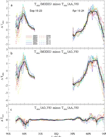
The color-coded lines in Fig. 8 interannually represent the differences in temperature among the three data sets for in-dividual years. The thick black lines indicated the yearly
dif-Figure 8. Zonal averaged values of (a) Tskin (MODIS) minus
Tskin(AA_V6), (b) Tskin(MODIS) minus Tskin(AO_V6), (c) Tskin
(AO_V6) minus Tskin (AA_V6) over the Northern Hemisphere
from 16 to 24 April 2003–2014, and over the Southern Hemisphere from 15 to 23 September 2003–2014. The values in each year rep-resent the corresponding color lines. The thick black line indicates the mean difference values.
ference averages. There was a significant degree of inter-annual variation in the difference between Tskin (MODIS)
and the two AIRS data sets (Fig. 8a–b). The variation was larger in 2009, 2010 and 2011 over the regions northward of 60◦N and southward of 55◦S where sea ice existed. Fig-ure 8b shows a value of Tskin(MODIS) minus Tskin(AO_V6)
that was similar to that in Fig. 8a. Tskin (MODIS) was
lower than Tskin(AO_V6) at the ice surface, but higher than Tskin (AO_V6) at the boundary of the sea ice. Figure 8c
showed the interannual variation of Tskin (AO_V6) minus Tskin (AA_V6). The interannual variation of the difference
between the AIRS retrievals was much larger in the high lat-itude than in the mid-latlat-itudes. The maximum difference of 1.56 K between the AIRS retrievals was found at 87–88◦N in 2011.
There could be several reasons for the observed differ-ences between Tskin(MODIS) and Tskin(AA_V6). The main
one can be attributed to the difference in the channel used for the retrievals of the skin temperature. The AIRS/AMSU
Table 3. The rate of the surface skin temperature change (K decade−1) of the MODIS, AIRS/AMSU, and AIRS only in each 10◦latitudinal belt over the Northern Hemisphere (NH) during 16–24 April and over the Southern Hemisphere (SH) during 15–23 September 2003–2014, using their colocated data in a 1◦×1◦grid. The ±values define the 95 % confidence intervals for the trends. The symbol “∗” means the significant value at a 95 % confidence interval. Note that the rates are subject to large uncertainty due to the short periods of the satellite-based temperature records.
Latitudinal MODIS AIRS/AMSU AIRS only MODIS minus MODIS minus AIRS only minus
belt AIRS/AMSU AIRS only AIRS/AMSU
< NH> 80–90◦N −0.558 ± 3.101 −0.100 ± 3.673 −0.093 ± 3.736 −0.458 −0.465 0.007 70–80◦N 2.302 ± 1.701∗ 2.826 ± 1.878∗ 2.711 ± 1.788∗ −0.524 −0.409 −0.115 60–70◦N −0.506 ± 1.173 −0.646 ± 1.294 −0.902 ± 1.050 0.140 0.396 −0.256 50–60◦N −0.345 ± 0.539 −0.522 ± 0.628 −0.466 ± 0.550 0.177 0.121 0.056 40–50◦N 0.292 ± 0.402 0.103 ± 0.576 0.191 ± 0.565 0.189 0.101 0.088 < SH> 50–60◦S 0.375 ± 0.400 0.315 ± 0.466 0.316 ± 0.600 0.060 0.059 0.001 60–70◦S −1.944 ± 2.271 −1.304 ± 1.890 −1.300 ± 1.918 −0.640 −0.644 0.004 70–80◦S −0.769 ± 2.687 −0.081 ± 2.586 −0.135 ± 2.633 −0.688 −0.634 −0.054
V6 only utilized shortwave window channels for the sur-face skin temperature, while the MODIS IST algorithm used the longwave window regions. The shortwave window could be mixed with the solar radiation during the daytime, but it was suitable for temperature sounding (Chahine, 1974, 1977; Susskind et al., 2014). The advantage of the longwave wdow was that its range corresponded to the peak of the in-frared radiation emitted from the earth (Prakash, 2000). On the other hand, the longwave window radiation could be af-fected more by clouds. In order to avoid cloud contamina-tion, the MODIS IST algorithm analyzed the pixel when the MODIS cloud mask was reported as clear sky (Hall et al., 2004). The MODIS cloud mask using visible reflectance had a high accuracy during the daytime, but a lower accuracy dur-ing the nighttime due to low illumination. As another reason for the temperature difference, Lee et al. (2013) suggested that there were substantial differences in observation time be-tween MODIS and AIRS in the high latitude regions, since the different scan angles of the two instruments resulted in different footprints, which could lead to the observed differ-ence in temperature. However, we suggested that the surface type classification method could be the primary reason for the temperature difference between the MODIS-based and AIRS-based data sets. AIRS/AMSU SST was retrieved af-ter the surface type was classified. On the other hand, the MODIS IST was calculated without the surface type classi-fication step. Then, the MODIS algorithm categorized pixels being ice if IST was less than the cutoff temperature. MODIS IST was calculated on the snow, sea ice, and ocean, assum-ing the surface was snow-covered (sea ice). The IST was uti-lized as a criterion for identifying the ice/water which might cause significant disagreement between the Tskin (MODIS)
and Tskin(AA_V6) in the range of 260–273 K.
4 Comparison of the surface skin temperature trends: IST vs. SST
In order to further investigate the effects of the difference among the satellite-observed temperatures from different measurement techniques or algorithms on the temperature anomaly trend, we calculated the trend in some latitude belts, using the three satellite-observed temperature data sets at each grid during 16–24 April 2003–2014 (in the Northern Hemisphere) and 15–23 September 2003–2014 in the South-ern Hemisphere. During this period, an unusually extensive surface melting event was observed in 2012 (Nghiem et al., 2012; Hall et al., 2013; Comiso and Hall, 2014).
Table 3 shows the temperature anomaly trend with a 95 % confidence level on the 10◦latitude belt. We arranged the data of MODIS IST, AIRS/AMSU, and AIRS only under the same condition in space and time. The signifi-cant warming trend in 70–80◦N was estimated in the fol-lowing order: AIRS/AMSU (2.83 K decade−1) > AIRS only (2.71 K decade−1) > Tskin (MODIS) (2.30 K decade−1). The
warming (0.10 to 0.38 K decade−1) at 40–50◦N and 50– 60◦S, and the cooling (−0.08 to −1.94 K decade−1) at 80– 90, 60–70, 50–60◦N, 60–70 and 70–80◦S of the three data sets occurred, but the trends were not significant. Comiso and Hall (2014) reported the SST trend using the Goddard Insti-tute for Space Studies (GISS) data set as 0.60 K decade−1
and the trend using the Advanced Very High Resolution Ra-diometer (AVHRR) data set as 0.69 K decade−1in the Arctic (> 64◦N) during 1981–2012. Our result in 70–80◦N, com-pared with the above studies, seems to indicate an accelera-tion in the Arctic warming.
The warming trend in the northern hemispheric high lat-itudes had been known to be caused in part by the well-known positive feedback among snow/ice, surface albedo
H.-J. Kang et al.: Uncertainties of satellite-derived surface skin temperatures in the polar oceans 4035 and temperature (Curry et al., 1995; Comiso and Hall,
2014). Tskin(MODIS) had a greater cooling tendency
com-pared to Tskin (AA_V6) in the higher latitude regions (70–
90◦N and 60–80◦S) (Table 3). The trend difference be-tween the two temperatures was −0.69 K decade−1 at 70– 80◦S. The trend difference of the Tskin (AA_V6) and Tskin
(AO_V6) (i.e., AIRS only minus AIRS/AMSU) was the largest (−0.26 K decade−1) at 60–70◦N. The cooling trend (−0.90 K decade−1) of the Tskin (AO_V6) was greater than
that (−0.65 K decade−1) of Tskin (AA_V6) at the latitude
band.
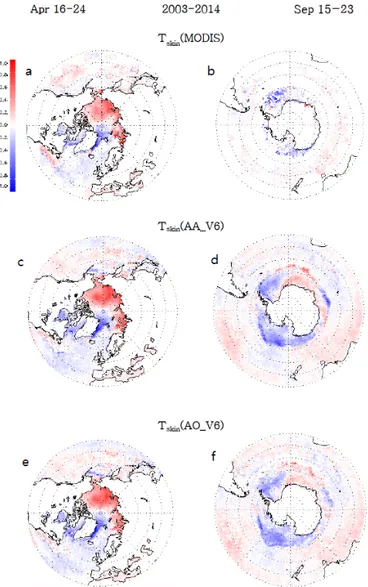
Figure 9a–b showed the SST anomaly trends from the
Tskin (MODIS) in a 1◦×1◦ grid over the Northern
Hemi-sphere during 16–24 April 2003–2014 and over the Southern Hemisphere during 15–23 September 2003–2014. The Tskin
(MODIS) trend was calculated on the grid, which had avail-able data that existed for over 10 years. Figure 9c–d and e–f showed the trend data for Tskin(AA_V6) and Tskin(AO_V6),
respectively, which all had 12-year data, individually. The trend distributions in all three of the data sets were similar over the Northern Hemisphere. Warming trend in the Beau-fort Sea, East Siberian Sea and Kara Sea was detected, while cooling was observed in the Hudson Bay and near Green-land. The significant warming trend appeared at 70–80◦N as shown in Table 3, and the trend based on the spatial distribu-tion varied depending on the regions (Fig. 9a, c and e). Ac-cording to Comiso and Hall (2014), a strong warming trend (> 1.5 K decade−1) existed near the Kara Sea and Baffin Bay among the entire Arctic, consistent with the noticeable trend revealed near the Kara Sea in our study. Over the Southern Hemisphere, there were not enough data to derive a trend for
Tskin(MODIS) mostly due to clouds. The trend analysis over
the sea ice regions from Tskin (AA_V6) and Tskin(AO_V6)
showed a strong cooling trend, especially near the Antarctic peninsula between the Weddell and Ross Seas (Fig. 9d and f). The cooling trend was generally dominant over the Southern Hemisphere. Marshall et al. (2014) suggested that based on the model experiments, the cooling trend around Antarctica as opposed to the warming trend around the Arctic Ocean was the result of the offset between the greenhouse gas and ozone hole responses, emphasizing the larger cooling effects associated with the Antarctic ozone hole.
The 12-year mean of the Tskin (MODIS) minus Tskin
(AA_V6) (Fig. 10a and c) and of the trend difference be-tween Tskin (MODIS) and Tskin (AA_V6) (Fig. 10b and d)
were compared in order to reveal the relationship between the temperature difference and the corresponding trend dif-ference over the Northern Hemisphere during 16–24 April 2003–2014 and over the Southern Hemisphere during 15– 23 September 2003–2014. Tskin (MODIS) was higher than Tskin (AA_V6) over the bays of Hudson and Baffin, and
Bering Sea (Fig. 10a). The warming trend of the Tskin
(MODIS) was also greater than that of the Tskin (AA_V6)
over the Hudson Bay and near the Kara Sea (Fig. 10b). The data for the trend difference in the Southern Hemisphere was
Figure 9. Satellite-derived 9-day anomaly trends (K yr−1)in a grid box of 1◦×1◦over the Northern Hemisphere during 16–24 April 2003–2014, for the (a) Tskin (MODIS), (c) Tskin (AA_V6), and (e) Tskin(AO_V6), and over the Southern Hemisphere during 16–
24 September 2003–2014, for the (b) Tskin (MODIS), (d) Tskin
(AA_V6), and (f) Tskin(AO_V6).
not sufficient due to the missing data of Tskin(MODIS) in the
cloudy condition (Fig. 10d).
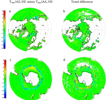
Figure 11 showed over both hemispheres the 12-year mean of the Tskin(AO_V6) minus Tskin(AA_V6) (Fig. 11a and c)
and the corresponding trend difference of the Tskin(AO_V6)
and Tskin(AA_V6) (Fig. 11b and d). The relationship of the
temperature difference and trend difference over the South-ern Hemisphere in Fig. 10 was hard to analyze due to the absence of a Tskin (MODIS) trend (Fig. 10c–d). However,
Fig. 11c–d clearly showed that the temperature difference had a significant impact on the trend difference over the Southern Hemisphere. The trend of the Tskin (AA_V6) and Tskin(AO_V6) agreed well except for at the region of the sea
Figure 10. (a) 12-year mean of Tskin (MODIS) minus Tskin
(AA_V6) (K) over the Northern Hemisphere during 16–24 April 2003–2014, and (b) difference in the thermal trend (K decade−1) between Tskin(MODIS) and Tskin(AA_V6). (c)–(d) are the same
as (a)–(b) except for over the Southern Hemisphere during 16– 24 September 2003–2014, respectively. (a) is the same as Fig. 3a in Kang and Yoo (2015).
ice boundary, implying that the algorithm identifying the sea ice affected the SST trend.
Uncertainties among satellite observations (Tskin
(MODIS), Tskin (AA_V6), and Tskin (AO_V6)) in the
sea ice region of the Northern Hemisphere are generally similar to those of the Southern Hemisphere in terms of zonal averages. However, the systematic difference between the observations can be more clearly seen in the latter region than in the former region due to more oceanic regions in the Southern Hemisphere (Figs. 10–11, and see also Fig. 7).
Table 4 quantitatively showed how the temperature differ-ences among the three types of SST affected each trend dif-ference over the hemispheric regions poleward either from 50◦N (shown in the left side of the table) during 16–24 April 2003–2014 or from 50◦S during 15–23 September 2003– 2014. In the upper portion, the average of the tempera-ture difference and the trend difference in the grid corre-sponding to the temperature difference condition was used, whereas the average values on the grids that had the same signs for the temperature difference and the trend differ-ence were used in the lower portion. Only the cases where grid number was greater than 100 were considered. The warmer temperature led to relatively warming trend, the cooler temperature led to relatively cooling trend. When the
Tskin(MODIS) was greater than Tskin(AA_V6) in the regions
poleward from 50◦S, the trend difference was in the reduced
Figure 11. Same as Fig. 10 except for Tskin(AO_V6) minus Tskin
(AA_V6). (a) is the same as Fig. 3c in Kang and Yoo (2015).
cooling trend (i.e., warmer direction) as −0.96, −0.66, and
−0.21 K decade−1with the conditions of Tskin(MODIS)
mi-nus Tskin(AA_V6) rising as more than 1, 1.5, and 2 K,
re-spectively. The uncertainty of the satellite-derived tempera-tures had a substantial effect on the uncertainty of the tem-perature trends. The data set has been reduced in the lower section of Table 4. The sample size can affect the estimated impact of 1T on 1Trend, but it looks like that the impact on the trends in the lower section is almost consistent with that in the upper section despite the reduced sample sizes.
5 Conclusions
The satellite-derived L3 products of MODIS IST and two SSTs from AIRS/AMSU and AIRS only were investigated with a comparative analysis during the vernal periods of 2003–2014: 16–24 April over the Northern Hemisphere and 15–23 September over the Southern Hemisphere. The origi-nal MODIS IST data were regridded onto a 1◦×1◦grid box for comparison with the AIRS retrievals. The difference be-tween the original MODIS IST and the converted one was within 0.5 K in a latitudinal belt.
The differences among the three types of satellite derived SST data were most prominent over the sea ice regions. Tskin
(MODIS) and Tskin (AA_V6) were comparable (r = 0.97–
0.99), but there was systematic disagreement occurred in the Tskin(MODIS) range of 260–273 K. The southern
hemi-spheric high latitude (60–90◦S) was the primary contributor to the disagreement between them. In comparison with the
H.-J. Kang et al.: Uncertainties of satellite-derived surface skin temperatures in the polar oceans 4037
Table 4. Uncertainties of the satellite-derived surface skin temperature rate (or trend; 1Trend) due to the temperature difference (1Tskin)
for the cases of Tskin(MODIS) minus Tskin(AA_V6) and Tskin(AO_V6) minus Tskin(AA_V6) in the upper portion of the table. Also, the
values of uncertainties provided in the lower portion of the table indicate the cases of ±1Trend with respect to ±1Tskin(double signs in the
same order). The uncertainties are not shown when the number of the grid (1◦×1◦) points (i.e., No. of grids in the table) is less than 100.
1Tskin(K) Poleward from 50◦N Poleward from 50◦S
Tskin(MODIS) vs. Tskin(AA_V6) Tskin(AO_V6) vs. Tskin(AA_V6) Tskin(MODIS) vs. Tskin(AA_V6) Tskin(AO_V6) vs. Tskin(AA_V6)
No. of 1Tskin 1Trend No. of 1Tskin 1Trend No. of 1Tskin 1Trend No. of 1Tskin 1Trend
grids (K decade−1) grids (K decade−1) grids (K decade−1) grids (K decade−1)
≥1.0 2155 2.01 −0.10 95 – – 425 2.01 −0.96 378 1.37 0.03 ≥1.5 1506 2.34 0.04 19 – – 253 2.25 −0.66 104 1.80 0.24 ≥2.0 940 2.71 0.19 5 – – 134 2.69 −0.21 22 – – ≤ −1.0 1839 −1.59 −0.45 236 −2.25 −0.34 224 −1.71 −0.43 877 −2.19 −0.37 ≤ −1.5 921 −1.94 −0.45 162 −2.72 −0.47 115 −2.18 −0.16 654 −2.52 −0.55 ≤ −2.0 367 −2.27 −0.60 109 −3.20 −0.78 55 – – 472 −2.82 −0.69 ≥1.0 912 2.15 1.21 40 – – 139 2.09 1.36 179 1.40 1.01 ≥1.5 707 2.41 1.22 8 – – 94 – – 51 – – ≥2.0 499 2.70 1.22 1 – – 64 – – 15 – – ≤ −1.0 1309 −1.59 −0.90 126 −2.51 −2.02 122 −1.69 −2.42 500 −2.26 −1.96 ≤ −1.5 643 −1.96 −0.92 89 – – 61 – – 387 −2.55 −2.06 ≤ −2.0 272 −2.28 −1.02 69 – – 27 – – 293 −2.81 −2.06
higher by up to 1.65 K than Tskin(AA_V6) on the boundary
of the sea ice/water, whereas it was lower by up to −2.04 K in the sea ice region.
The spatial correlation coefficients (0.992–0.999) of the Tskin (AO_V6) and Tskin (AA_V6) over both
hemi-spheres were greater than those (0.968–0.994) between Tskin
(MODIS) and Tskin(AA_V6). The Tskin(AO_V6) compared
to the Tskin(AA_V6) had a bias of 0.168 K with a RMSE of
0.590 K over the Northern Hemisphere high latitudes and a bias of −0.109 K with a RMSE of 0.852 K over the southern hemispheric high latitudes. There was a systematic disagree-ment between the Tskin (AA_V6) and Tskin (AO_V6) at the
sea ice boundary. It is likely due to the fact that the AIRS only algorithm utilized a less accurate GCM forecast than the microwave data over the seasonally varying frozen oceans.
The temperature differences among the three types of data sets showed a high degree of interannual variations over the latitudinal belts where sea ice existed. The significant warming rates (2.3 ± 1.7 ∼ 2.8 ± 1.9 K decade−1) were re-vealed by all three data sets in the northern hemispheric high-latitude regions (70–80◦N) could be interpreted as the ice-albedo feedback. The discrepancies between the trends of the Tskin(AA_V6) and Tskin(AO_V6) occurred at the sea ice
boundary. When the Tskin(AA_V6) trends were compared to
those of the Tskin (MODIS) or Tskin (AO_V6) in a 1◦×1◦
grid, the warmer temperature difference tended to lead to a relative warming trend, whereas the cooler temperature dif-ference tended to lead to a relative cooling trend.
The systematic disagreement between the Tskin(MODIS)
and Tskin(AA_V6) could be caused by (1) the channels used
for the surface skin temperature, (2) the cloud contamina-tion, (3) the difference in local time of observation between the MODIS and AIRS, and (4) the surface type classifica-tion method. Whereas the AIRS/AMSU V6 used only the
shortwave window channels for the surface skin tempera-ture, MODIS IST used the longwave window regions. The MODIS IST product utilized the MODIS cloud mask with visible reflectance, which had lower accuracy during the night (Hall et al., 2004). Lee et al. (2013) reported that the local times of observation between the MODIS and AIRS were almost the same from 60◦N–60◦S, but they were quite different in the high latitude regions. It is likely that the main cause to the observed SST differences near the sea ice boundary was in the way the surface type was classified. The AIRS/AMSU algorithm conjugated the emissivity dif-ference in the low and high frequency microwave bands (23 and 50 GHz) in order to identify sea ice. However, MODIS IST was calculated without the surface type classification.
The AIRS/AMSU L2 data offer the surface type (coast-line, land, ocean, two types of sea ice, two types of snow, and glacier/snow), and the AIRS/AMSU L3 data provide the number of these various surface types in a grid. The AIRS only L2 also offer the surface type (coastline, land, ocean, two types of sea ice, and snow), and its L3 data provide the number of these various surface types in a grid. Under the condition without ground truth, the direct validation has a limit because the surface classifications of AIRS/AMSU and AIRS only have some difference. Although the AIRS only has utilized the forecast surface temperature from the GFS, there is a good agreement in SST between AIRS/AMSU and AIRS only in most regions. However, the disagreement be-tween them over the land regions of the Sahara desert, parts of Spain and in the US with snow cover at night has been reported (Dang et al., 2012).
We have investigated the effect in the difference of spa-tial resolution between L2 and L3 products, utilizing the L2 products (Tskin (MODIS), Tskin (AA_V6), and Tskin
among the three L2 data sets are similar to those of the L3, but the magnitude of Tskin (MODIS) minus Tskin (AA_V6)
for L2 data sets is somewhat different from that for the L3 data sets (not shown). Based on the L3 products in this study, it seems to be sufficient to allow us to show the system-atic characteristics of the uncertainties. Although the detailed analysis of L2 is beyond the scope of this study, further stud-ies are warranted.
The SST in the polar region is a useful parameter being used to derive the climate change signal, although it has been challenging to measure an accurate SST. Based on our results from detailed comparative investigation, we cautiously sug-gested that the observed difference and uncertainty among the satellite-derived SSTs were likely caused by the differ-ent sea ice detecting methods used in each algorithm. This study suggested that the ice forecast derived from other mi-crowave satellite data could improve the AIRS only prod-uct from the better accuracy of surface classification. In ad-dition, the methods also affected the temperature trend. In this study, we aimed to help in understanding characteristics of the infrared and microwave measurements for the surface skin temperature, and the method for identifying sea ice. We believe the results of this study can be useful for the inter-pretation and the modeling of the climate change associated with the temperature trends.
H.-J. Kang et al.: Uncertainties of satellite-derived surface skin temperatures in the polar oceans 4039 Appendix A:
Figure A1. The difference values (a) between Tskin(MODIS) and Tskin(AA_V6), and (b) Tskin(AA_V6) and Tskin(AO_V6) over a possibly
frozen region; shown in Fig. 7. The 5 % significance level is presented as grey solid lines, and the shaded areas are statistically significant at the 0.05 level.
Acknowledgements. This study was supported by the National
Research Foundation of Korea (NRF) grant funded by the Korean Government (MSIP) (No. 2009-0083527) and the Ko-rean Ministry of Environment as the Eco-technopia 21 project (No. 2012000160003). We thank Goddard Earth Sciences Data Information and Services Center for AIRS/AMSU data, and NASA National Snow and Ice Data Center for MODIS IST data. We also thank Bob Iacovazzi Jr., J. M. Blaisdell, and C.-Y. Liu for their constructive comments.
Edited by: B. Kahn
References
Aumann, H. H., Chahine, M. T., Gautier, C., Goldberg, M. D., Kalnay, E., McMillin, L. M., Revercomb, H., Rosenkranz, P. W., Smith, W. L., Staelin, D. H., Strow, L. L., and Susskind, J.: AIRS/AMSU/HSB on the Aqua mission: Design, science objectives, data products, and processing systems, IEEE IEEE T. Geosci. Remote, 41, 253–264, doi:10.1109/tgrs.2002.808356, 2003.
Barnes, W. L., Pagano, T. S., and Salomonson, V. V.: Prelaunch characteristics of the Moderate resolution Imaging Spectrora-diometer (MODIS) on EOS-AM1, IEEE T. Geosci. Remote, 36, 1088–1100, doi:10.1109/36.700993, 1998.
Boucher, O., Randall, D., Artaxo, P., Bretherton, C., Feingold, G., Forster, P., Kerminen, V.-M., Kondo, Y., Liao, H., Lohmann, U., Rasch, P., Satheesh, S. K., Sherwood, S., Stevens, B., and Zhang, X. Y.: Clouds and Aerosols, in: Climate change 2013: The physical science basis, Contribution of working group I to the fifth assessment report of the intergovernmental panel on cli-mate change, edited by: Stocker, T. F., Qin, D., Plattner, G.-K., Tignor, M., Allen, S. K., Boschung, J., Nauels, A., Xia, Y., Bex, V., and Midgley, P. M., Cambridge University Press, Cambridge, UK, 571–657, 2013.
Chahine, M. T.: Remote sounding of cloudy atmospheres. I. The single cloud layer, J. Atmos. Sci., 31, 233–243, doi:10.1175/1520-0469(1974)031<0233:RSOCAI>2.0.CO;2, 1974.
Chahine, M. T.: Remote sounding of cloudy atmospheres. II. Multiple cloud formations, J. Atmos. Sci., 34, 744–757, doi:10.1175/1520-0469(1977)034<0744:RSOCAI>2.0.CO;2, 1977.
Comiso, J. C. and Hall, D. K.: Climate trends in the Arctic as ob-served from space, Wiley Interdiscip. Rev.-Clim. Chang., 5, 389– 409, doi:10.1002/wcc.277, 2014.
Comiso, J. C. and Stock, L. V.: Studies of Antarctic cloud cover variability from 1982 through 1999, Geoscience and Remote Sensing Symposium, 2001, IGARSS ’01, IEEE 2001 Interna-tional, 1782–1785, 2001.
Curry, J. A., Schramm, J. L., and Ebert, E. E.: Sea ice-albedo climate feedback mechanism, J. Clim., 8, 240–247, doi:10.1175/1520-0442(1995)008<0240:SIACFM>2.0.CO;2, 1995.
Dang, H. V. T., Lambrigtsen, B., and Manning, E.: AIRS/AMSU/HSB version 6 level 2 performance and test report, available at: http://disc.sci.gsfc.nasa.gov/AIRS/documentation/
v6_docs/v6releasedocs-1/V6_L2_Performance_and_Test_ Report.pdf (last access: 8 June 2015), 2012.
Dong, S. F., Gille, S. T., Sprintall, J., and Gentemann, C.: Val-idation of the Advanced Microwave Scanning Radiometer for the Earth Observing System (AMSR-E) sea surface temperature in the southern ocean, J. Geophys. Res.-Oceans, 111, C04002, doi:10.1029/2005jc002934, 2006.
Donlon, C. J., Minnett, P. J., Gentemann, C., Nightingale, T. J., Bar-ton, I. J., Ward, B., and Murray, M. J.: Toward improved val-idation of satellite sea surface skin temperature measurements for climate research, J. Clim., 15, 353–369, doi:10.1175/1520-0442(2002)015<0353:tivoss>2.0.co;2, 2002.
Emery, W. J., Castro, S., Wick, G. A., Schluessel, P., and Donlon, C.: Estimating sea surface temperature from infrared satellite and in situ temperature data, Bull. Amer. Meteorol. Soc., 82, 2773– 2785, doi:10.1175/1520-0477(2001)082<2773:esstfi>2.3.co;2, 2001.
Gardner, M. W. and Dorling, S. R.: Artificial neural networks (the multilayer perceptron) – A review of applications in the atmospheric sciences, Atmos. Environ., 32, 2627–2636, doi:10.1016/s1352-2310(97)00447-0, 1998.
Grody, N., Weng, F., and Ferraro, R.: Application of AMSU for obtaining water vapor, cloud liquid water, precipitation, snow cover and sea ice concentration, in: Technical proceedings of the tenth international atovs study conference, Colorado, USA, 27 January–2 February 1999, 230–240, 1999.
Hall, D. K. and Riggs, G. A.: Accuracy assessment of the MODIS snow products, Hydrol. Process., 21, 1534–1547, doi:10.1002/hyp.6715, 2007.
Hall, D. K. and Riggs, G. A.: MODIS/Terra Sea Ice Extent and IST Daily L3 Global 4 km EASE-Grid Day, Version 6, Subset used: 16–24 April and 15–23 September 2003–2015, Boulder, Colorado, USA, NASA DAAC at the National Snow and Ice Data Center, available at: http://nsidc.org/data/docs/daac/modis/ mod29e1d/index.html (updated daily), last access: 29 June, 2015. Hall, D. K., Key, J. R., Casey, K. A., Riggs, G. A., and Cavalieri, D. J.: Sea ice surface temperature product from MODIS, IEEE T. Geosci. Remote, 42, 1076–1087, doi:10.1109/tgrs.2004.825587, 2004.
Hall, D. K., Comiso, J. C., DiGirolamo, N. E., Shuman, C. A., Box, J. E., and Koenig, L. S.: Variability in the surface temperature and melt extent of the Greenland ice sheet from MODIS, Geophys. Res. Lett., 40, 2114–2120, doi:10.1002/grl.50240, 2013. Hewison, T. J. and English, S. J.: Airborne retrievals of snow and
ice surface emissivity at millimeter wavelengths, IEEE T. Geosci. Remote, 37, 1871–1879, doi:10.1109/36.774700, 1999. Jakob, C.: Cloud cover in the ECMWF reanalysis, J. Clim., 12, 947–
959, doi:10.1175/1520-0442(1999)012<0947:cciter>2.0.co;2, 1999.
Jin, M., Dickinson, R. E., and Vogelmann, A. M.: A comparison of CCM2–BATS skin temperature and surface-air temperature with satellite and surface observations, J. Clim., 10, 1505–1524, doi:10.1175/1520-0442(1997)010<1505:ACOCBS>2.0.CO;2, 1997.
Kang, H.-J. and Yoo, J.-M.: Uncertainties of satellite-observed surface skin temperatures due to sea ice in the Arctic ocean: MODIS, AIRS/AMSU and AIRS Only, J. Korean Earth Sci. Soc., 36, 139–157, doi:10.5467/JKESS.2015.36.2.139, 2015 (in Korean).
H.-J. Kang et al.: Uncertainties of satellite-derived surface skin temperatures in the polar oceans 4041
Key, J. R., Collins, J. B., Fowler, C., and Stone, R. S.: High-latitude surface temperature estimates from thermal satellite data, Remote Sens. Environ., 61, 302–309, doi:10.1016/S0034-4257(97)89497-7, 1997.
Knuteson, R., Cychosz, J., Lee, S. C., Revercomb, H., Tobin, D., and Vinson, K.: Comparison of LST from AIRS and MODIS from the EOS Aqua platform, 10th symposium on Integrated Ob-serving and Assimilation Systems for the Atmosphere, Oceans, and Land Surface (IOASAOLS), the 86th AMS annual meeting, Atlanta, USA, 28 January–3 February 2006, P2.2, 2006. Kongoli, C., Boukabara, S., Yan, B., Weng, F., and Ferraro, R.:
Sea ice concentration retrievals from variationally retrieved mi-crowave surface emissivities, available at: http://microrad2008. cetem.org/public/presentations/20080314_16.50_Kongoli.pdf (last access: 4 December 2014), 2008.
Lachlan-Cope, T.: Antarctic clouds, Polar Res., 29, 150–158, doi:10.1111/j.1751-8369.2010.00148.x, 2010.
Lee, Y.-R., Yoo, J.-M., Jeong, M.-J., Won, Y.-I., Hearty, T., and Shin, D.-B.: Comparison between MODIS and AIRS/AMSU satellite-derived surface skin temperatures, Atmos. Meas. Tech., 6, 445–455, doi:10.5194/amt-6-445-2013, 2013.
Li, J., Liu, C. Y., Zhang, P., and Schmit, T. J.: Applications of full spatial resolution space-based advanced infrared soundings in the preconvection environment, Wea. Forecasting, 27, 515–524, doi:10.1175/WAF-D-10-05057.1, 2012.
Liou, K. N.: An introduction to atmospheric radiation, Academic Press, Amsterdam; Boston, 583 pp., 2002.
Liu, C. Y., Li, J., Weisz, E., Schmit, T. J., Ackerman, S. A., and Huang, H. L.: Synergistic use of AIRS and MODIS radiance measurements for atmospheric profiling, Geophys. Res. Lett., 35, L21802, doi:10.1029/2008gl035859, 2008.
Liu, C. Y., Liu, G. R., Lin, T. H., Liu, C. C., Ren, H., and Young, C. C.: Using surface stations to improve sounding retrievals from hyperspectral infrared instruments, IEEE T. Geosci. Remote, 52, 6957–6963, doi:10.1109/tgrs.2014.2305992, 2014.
Marshall, J., Armour, K. C., Scott, J. R., Kostov, Y., Hausmann, U., Ferreira, D., Shepherd, T. G., and Bitz, C. M.: The ocean’s role in polar climate change: asymmetric Arctic and Antarctic responses to greenhouse gas and ozone forcing, Phil. Trans. R. Soc., 372, 20130040, doi:10.1098/rsta.2013.0040, 2014.
Molnar, G. I. and Susskind, J.: Validation of AIRS/AMSU cloud retrievals using MODIS cloud analyses, in: Proc. SPIE 5806, Al-gorithms and Technologies for Multispectral, Hyperspectral, and Ultraspectral Imagery XI, 13 July 2005, 618–629, 2005. Nghiem, S. V., Hall, D. K., Mote, T. L., Tedesco, M., Albert, M. R.,
Keegan, K., Shuman, C. A., DiGirolamo, N. E., and Neumann, G.: The extreme melt across the Greenland ice sheet in 2012, Geophys. Res. Lett., 39, L20502, doi:10.1029/2012gl053611, 2012.
Olsen, E.: AIRS/AMSU/HSB version 6 changes from version 5, available at: http://disc.sci.gsfc.nasa.gov/AIRS/documentation/ v6_docs/v6releasedocs-1/V6_Changes_from_V5.pdf (last ac-cess: 4 December 2014), 2013a.
Olsen, E.: AIRS/AMSU/HSB version 6 retrieval flow, avail-able at: http://disc.sci.gsfc.nasa.gov/AIRS/documentation/v6_ docs/v6releasedocs-1/V6_Retrieval_Flow.pdf (last access: 4 De-cember 2014), 2013b.
Prakash, A.: Thermal remote sensing: concepts, issues and applica-tion, XIXth ISPRS Congress, Amsterdam, the Netherlands, 239– 243, 2000.
Riggs, G. A., Hall, D. K., and Ackerman, S. A.: Sea ice extent and classification mapping with the Moderate resolution Imag-ing Spectroradiometer airborne simulator, Remote Sens. Envi-ron., 68, 152–163, doi:10.1016/s0034-4257(98)00107-2, 1999. Riggs, G. A., Hall, D. K., and Salomonson, V. V.: MODIS sea
ice products user guide to collection 5, available at: http:// modis-snow-ice.gsfc.nasa.gov/uploads/siug_c5.pdf (last access: 7 February 2015), 2006.
Scott, K. A., Li, E., and Wong, A.: Sea ice surface temper-ature estimation using MODIS and AMSR-E data within a guided variational model along the Labrador Coast, IEEE J. Sel. Top. Appl. Earth Observ. Remote Sens., 7, 3685–3694, doi:10.1109/jstars.2013.2292795, 2014.
Susskind, J., Blaisdell, J. M., Iredell, L., and Keita, F.: Im-proved temperature sounding and quality control methodol-ogy using AIRS/AMSU Data: The AIRS science team version 5 retrieval algorithm, IEEE T. Geosci. Remote, 49, 883–907, doi:10.1109/tgrs.2010.2070508, 2011.
Susskind, J., Blaisdell, J. M., and Iredell, L.: Improved methodol-ogy for surface and atmospheric soundings, error estimates, and quality control procedures: the atmospheric infrared sounder sci-ence team version-6 retrieval algorithm, APPRES, 8, 084994, doi:10.1117/1.JRS.8.084994, 2014.
Tian, B. J., Fetzer, E. J., Kahn, B. H., Teixeira, J., Manning, E., and Hearty, T.: Evaluating CMIP5 models using AIRS tropospheric air temperature and specific humidity climatology, J. Geophys. Res.-Atmos., 118, 114–134, doi:10.1029/2012jd018607, 2013. Tobin, D. C., Revercomb, H. E., Knuteson, R. O., Lesht, B. M.,
Strow, L. L., Hannon, S. E., Feltz, W. F., Moy, L. A., Fetzer, E. J., and Cress, T. S.: Atmospheric radiation measurement site at-mospheric state best estimates for atat-mospheric infrared sounder temperature and water vapor retrieval validation, J. Geophys. Res.-Atmos., 111, D09S14, doi:10.1029/2005jd006103, 2006. von Storch, H. and Zwiers, F. W.: Statistical Analysis in Climate
Research, Cambridge University Press, Cambridge, UK, 484 pp., 1999.
Wilks, D. S.: Statistical methods in the atmospheric sciences, Aca-demic Press, San Diego, 467 pp., 1995.
Won, Y.-I.: Readme document for AIRS Level-3 version 5 stan-dard products: daily (AIRH3STD, AIRX3STD, AIRS3STD), 8-day (AIRH3ST8, AIRX3ST8, AIRS3ST8) & monthly (AIRH3STM, AIRX3STM, AIRS3STM), available at: http://disc.sci.gsfc.nasa.gov/TRMM/AIRS/documentation/ readmes/README.AIR-3ST.pdf (last access: 4 December 2014), 2008.
Yoo, J.-M., Won, Y.-I., Jeong, M.-J., Kim, K.-M., Shin, D.-B., Lee, Y.-R., and Cho, Y.-J.: Intensity of climate variability de-rived from the satellite and MERRA reanalysis temperatures: AO, ENSO, and QBO, J. Atmos. Sol.-Terr. Phys., 95–96, 15–27, doi:10.1016/j.jastp.2013.01.002, 2013.
Zheng, J., Li, J., Schmit, T., Li, J., and Liu, Z.: The impact of AIRS atmospheric temperature and moisture profiles on hurricane fore-casts: Ike (2008) and Irene (2011), Adv. Atmos. Sci., 32, 319– 335, doi:10.1007/s00376-014-3162-z, 2015.