1. INTRODUCTION
Some researchers suggest a model of fuzzy neuron that linear synaptic connections can be replaced with a nonlinearity characterized by a membership function and a fuzzy neural network model [1], [2]. The nonlinear characteristics of which are represented by fuzzy if-then rules with complementary membership functions. Since neo fuzzy neuron model or fuzzy neural network can have a good ability to describe a nonlinear relationship between multi-inputs and multi-output as well as its short leaning time compared with a conventional neural network, they are expecting as future linguistic tool for intelligence or soft computing. On the other hand, radial basis function networks (RBFNs) and back propagation neural networks (BPNNS) have yielded useful results in many practical areas such as pattern recognition, system identification and control, due primarily to their simple structures for realization and well established training algorithms. Many fuzzy paradigms, meanwhile, have been studied is recent years by viewing a fuzzy logic system (FLS) as a functionally equivalent RBFN or BPNN. As indicated in some papers [3], [4], the most important advantage of such an FLS spanned by fuzzy basic functions is the provision of a natural framework for combining numerical values and linguistic symbols in a uniform way. From a mathematical point of view, the input-output expressions of those mappings are identical in spite of the distinct inference procedure. Capability discrimination between neural and fuzzy system is thus diminished for proofs of universal neural/fuzzy approximators. Using neural networks or fuzzy systems to approximate a given plant or to control a process flow depends on whether rich available data are at hand or whether the 'If-Then' control heuristics could be established by human experts familiar with system dynamics under consideration. A simple sigmoidal-like neuron is employed as a preassigned algorithm of the law of structural change which is directed by the current value of the error signal. However, in case of almost fuzzy logic, fuzzy-neural network, grade of membership and weighting function must be tuned by an approximation or experience-based tuning method. Some papers are written with a couple of objectives to demonstrate
that genetic algorithms (GAs) are an efficient and robust tool for generating fuzzy rules and weighting function. GAs can construct a set of fuzzy rules that optimize multiple criteria [5]. An important observation that the rules searched by GAs are randomly scattered is made and a solution to this problem is provided by including a smoothness cost in the objective function.
On the other hand, the particle swarm is an algorithm for finding optimal regions of complex search spaces through interaction of individuals in a population of particles. Though the algorithm, which is based on a metaphor of social interaction, has been shown to perform well, researchers have not adequately explained how it works. Further, traditional versions of the algorithm have had some dynamical properties that were not considered to be desirable, notably the particles’ velocities needed to be limited in order to control their trajectories.
This paper proposes particle swarm optimization algorithm based optimal learning approach of fuzzy-neural network [1-5]. The first phase of the PSOA-FNN is to find the initial membership functions of the fuzzy neural network model and the second phase is to obtain optimal membership functions of the proposed model by particle swarm optimization algorithm.
2. STRUCTURE OF A PARTICLE SWARM
OPTIMIZATION ALGORITHM BASED
FUZZY-NEURAL NETWORK
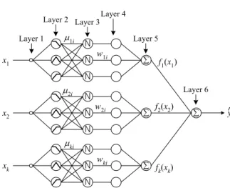
The structure of PSOA-FNN is shown in Fig. 1 [3] and the output of the FNN part of PSOA-FNN can be represented by the following equation (1).
In Fig. 1 and Equation (1), the input space x is divided i into several fuzzy segments which are characterized by membership functions µi1,µi2,...,µin within the range between xmin and xmax . The grade of membership function is also given as numbers assigned to labels of fuzzy membership function. The membership functions are followed by variable weights wi1,...win. Mapping from xi to
) ( i i x
f is determined by fuzzy inferences and fuzzy rule is
Optimal Learning of Fuzzy Neural Network Using Particle Swarm
Optimization Algorithm
Dong Hwa Kim, Jae Hoon Cho
Dept. of Instrumentation and Control Eng., Hanbat National University, 16-1 San Duckmyong-Dong Yuseong-Gu, Daejon City, Korea, 305-719.
E-mail: [email protected], Hompage: aialab.net Tel: +82-42-821-1170, Fax: +82-821-1164
Abstract: Fuzzy logic, neural network, fuzzy-neural network play an important as the key technology of linguistic modeling for intelligent control and decision making in complex systems. The fuzzy-neural network (FNN) learning represents one of the most effective algorithms to build such linguistic models. This paper proposes particle swarm optimization algorithm based optimal learning fuzzy-neural network (PSOA-FNN). The proposed learning scheme is the fuzzy-neural network structure which can handle linguistic knowledge as tuning membership function of fuzzy logic by particle swarm optimization algorithm. The learning algorithm of the PSOA-FNN is composed of two phases. The first phase is to find the initial membership functions of the fuzzy neural network model. In the second phase, particle swarm optimization algorithm is used for tuning of membership functions of the proposed model.
Keywords: Fuzzy neural network; Particle swarm algorithm; Multiobjective control; Optimization.
defined as Equation (2). x1 y^ µ1i N N N ∑ w1i f1(x1) ∑ x2 N N N ∑ xk N N N ∑ µ2i w2i µki wki f2(x2) fk(xk) Layer 2 Layer 3Layer 4
Layer 1 Layer 5
Layer 6
Fig. 1. The structure of particle swarm optimization algorithm based optimal learning fuzzy-neural network.
∑
= = + + + = m i i i m m x f x f x f x f y 1 2 2 1 1 ) ( ) ( ... ) ( ) ( (1) xn yxn in i n x yx i i w C then A is x If R w C then A is x If R = • • • = : : 1 1 1 1 (2) As the fuzzy inferences adopted here is that of a singleton consequent, each weight w is a deterministic value such as ij 0.8, 0.9. It should be emphasized that each membership function in antecedent is triangular and assigned to be complementary (so called by the authors) with neighbouring ones. In other words, an input signali
x activates only two membership functions simultaneously and the sum of grades of these two neighbouring membership functions labelled by k and k+1 is always equal to 1, that is .µi,k(xi)+µi,k+1(xi)=1 So, the output of the fuzzy neural network can be represented by the following simple Equation (3). xi n i xi i k i i ik ik i ik ik i ik n j i ij n j ij i ij n i yxi xi i i w x x w x w x x w x C x f
∑
∑
∑
∑
= + + + = = = ⋅ = + + = = • = 1 1 , 1 1 1 1 1 ) ( ) ( ) ( ) ( ) ( ) ( ) (µ
µ
µ
µ
µ
µ
µ
µ
(3)In this Equation, the weight w are assigned by learning ij
the rule of which is described by n if-then rules. That is, If input xi lies in the fuzzy segment µij , then the corresponding weight wij should be increased directly proportional to the output error (y- y ), because the error is caused by the weight. This proposition can be represented by the following equation;
1 1( ) ) ( ) ( i = xi i xi+ xi+ i xi+ i x x w x w f
µ
µ
(4)The learning procedure is the incremental change of weights for each input pattern. That is, the incremental change of minimizing the squared error (4) is obtained from
( )
(
() ( 1))
2 ) 1 ( + = − + − − ∆wxi t δ y yµxi αi wxi t wxi t (5) In this learning algorithm, all the initial weights are assigned to be zero and the updating of the weights is achieved after calculation of cumulative value in Equation (5).Where, y is the given data, y is the output of model,
δlearning rate, α is momentum constant and δ,α have the range of 0 to 1, respectively. The wxi is the present weighting function and wxi(t−1) is the previous weighting function.
3. PARTICLE SWARM OPTIMIZATION
ALGORITHMS FOR OBTAINING OPTIMAL
LEARNING OF THE FNN
3.1 Overview of Particle Swarm Optimization Algorithm
A population of particles is initialized with random positions xri and velocities vri , and a function, f, is evaluated, using the particle’s positional coordinates as input values. Positions and velocities are adjusted, and the function evaluated with the new coordinates at each time-step. When a particle discovers a pattern that is better than any it has found previously, it stores the coordinates in a vectorPri. The difference between Pi
r
(the best point found by i so far) and the individual’s current position is stochastically added to the current velocity, causing the trajectory to
oscillate around that point. Further, each particle is defined within the context of a topological neighborhood comprising itself and some other particles in the population. The stochastically weighted difference between the neighborhood’s best position Prg and the individual’s current position is also added to its velocity, adjusting it for the next time-step. These adjustments to the particle’s movement through the space cause it to search around the two best positions.
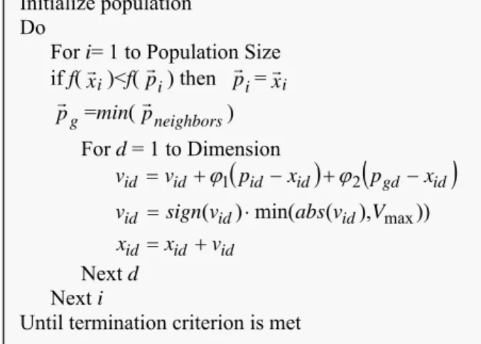
The algorithm in pseudocode as the following figures [7-11]:
Fig. 2. Procedure for particle swarm optimization algorithm.
The variables ϕ1 and ϕ2 are random positive numbers,
drawn from a uniform distribution and defined by an upper limit ϕmax which is a parameter of the system. In this version, the term variable vid is limited to the range
max
V
values of the elements in Pg r
are determined by comparing the best performances of all the members of i’s topological neighborhood, defined by indexes of some other population members, and assigning the best performer’s index to the variable g. Thus Pg
r
represents the best position found by any member of the neighborhood.
The random weighting of the control parameters in the algorithm results in a kind of explosion or a “drunkard's walk” as particles’ velocities and positional coordinates careen toward infinity. The explosion has traditionally been contained through implementation of a Vmax parameter, which limits step-size, or velocity. The current paper however demonstrates that the implementation of properly defined constriction coefficients can prevent explosion; further, these coefficients can induce particles to converge on local optima.
An important source of the swarm’s search capability is the interactions among particles as they react to one another’s findings. Analysis of interparticle effects is beyond the scope of this paper, which focuses on the trajectories of single particles.
We begin the analysis by stripping the algorithm down to a most simple form; we will add things back in later. The particle swarm formula adjusts the velocity vri by adding two terms to it. The two terms are of the same form, that is,
(
pr −xri)
ϕ
, where Pris the best position found so far, by the individual particle in the first term, or by any neighbor in the second term. The formula can be shortened by redefiningpid as follows: 2 1 2 1
ϕ
ϕ
ϕ
ϕ
+ + ← p p pid id gd (6)Thus we can simplify our initial investigation by looking at the behavior of a particle whose velocity is adjusted by only one term:
( )
t v( )
t(
p x( )
t)
vid +1 = id +
ϕ
id − id , (7)where ϕ=ϕ1+ϕ2 This is algebraically identical to the standard two-term form.
When the particle swarm operates on an optimization problem, the value of Pi
r
is constantly updated, as the system evolves toward an optimum. In order to further simplify the system and make it understandable, we set Pi
r
to a constant value in the following analysis. The system will also be more understandable if we make ϕ a constant as well; where normally it is defined as a random number between zero and a constant upper limit, we will remove the stochastic component
initially and reintroduce it in later sections. The effect of ϕ on the system is very important, and much of the present paper is involved in analyzing its effect on the trajectory of a particle.
The system can be simplified even further by considering a 1-dimensional problem space, and again further by reducing the population to one particle. Thus we will begin by looking at a stripped-down particle by itself, e.g., a population of one, one-dimensional, deterministic particle, with a constant p.
Thus we begin by considering the reduced system:
( )
(
)
) 1 ( ) ( ) 1 ( ) ( ) 1 ( ⎩ ⎨ ⎧ + + = + − + = + t v t x t x t x p t v t vϕ
(8)where p and ϕ are constants. No vector notation is necessary, and there is no randomness.
Kennedy [11] found that the simplified particle’s trajectory is dependent on the value of the control parameter ϕ, and recognized that randomness was responsible for the explosion of the system, though the mechanism which caused the explosion was not understood. M. clerc [10] further analyzed the system and concluded that the particle as seen in discrete time on an underlying continuous foundation of sine waves.
The present paper analyzes the particle swarm as it moves in discrete time (the algebraic view), then progresses to the view of it in continuous time (the analytical view). A 5-dimensional depiction is developed, which completely describes the system. These analyses lead to a generalized model of the algorithm, containing a set of coefficients to control the system’s convergence tendencies. When randomness is re-introduced to the full model with constriction coefficients, the deleterious effects of randomness are seen to be controlled. Some results of the particle swarm optimizer, using modifications derived from the analysis, are presented; these results suggest methods for altering the original algorithm in ways that eliminate some problems and increase the optimization power of the particle swarm.
3.2 Particle Swarm Optimization Based Membership Function Tuning
In this paper, when the initial value of the membership function type of triangular as Figs. 3, 4 are given by X1_min=[0.46, 0.48], X1_max=[0.77, 0.81], X2_min=[45.0, 47.0] X2_max=[ 61.0, 63.0], and learning rate boundary δ =[0.001, 0.01], momentum constant boundary α=[0.00001, 0.0004], respectively, the final membership function obtained by particle swarm optimization algorithm is dashed line as shown in Fig. 3 and Fig. 4.
0 . 4 8 0 .4 6
0 .4 7 9 9 6 7 7 4 6 7 0 .7 7 8 9 4 5 7 4 0 6
0 . 7 7 0 .8 1
, Fig. 3. Membership function shape of x1.
4 7 .0
4 6 .2 4 7 5 0 0 6 5 5
6 1 . 0 6 3 .0
6 2 .2 5 6 3 0 4 9 8 5 3
Fig. 4. Membership function shape of x1.
Initialize population
Do
For i= 1 to Population Size
if f(
xri)<f( p
r ) then p
ir =
ix
r
ip
gr =min( p
r
neighbors)
For d = 1 to Dimension
(
id id)
(
gd id)
id id v p x p x v = +ϕ
1 − +ϕ
2 − )) ), ( min( ) (v
abs
v
V
maxsign
v
id = id ⋅ id id id idx
v
x
= +Next d
Next i
3.3 Particle Swarm Optimization Algorithm Based Computational Procedure for Optimal Selection of Parameter
In this algorithm, we use the particle swarm optimization algorithm based calculation procedure shown in Fig. 2 to optimize the learning rate, momentum term and fuzzy membership function of the above PSOA-FNN. We use 10 generation and 100 generation, 60 populations, 10 bits per string, crossover rate equal to 0.6, and mutation probability equal to 0.1, respectively.
The searching procedures of the proposed PSOA-FNN structure is shown as below.
[Step 1] Specify the lower and upper bounds of the six parameters of fuzzy-neural network structure and initialize randomly the individuals of the population including searching points, velocities, pbests, and gbest.
[Step 2] Calculate the evaluation value of each individual in
the population using the evaluation function given by ) ( 1 i x W f = .
The evaluation function is a reciprocal of the performance criterion as in (9). It implies the smaller the value of individual , the higher its evaluation value. In order to limit the evaluation value of each individual of the population within a reasonable range.
These performance criteria in the time domain include the specification for tuning. The performance criterion can satisfy the designer requirements using the weighting factor value. We can set to be larger than 0.7. On the other hand, we can set to be smaller than 0.7 to reduce the over fitting. In this paper, is set in the range of 0.8 to 1.5.
[Step 3] Compare each individual’s evaluation value with its pbests. The best evaluation value among the is denoted as gbest.
[Step 4] Modify the member velocity of each individual according to (9)
(
)
(
)
6
,...,
2
,
1
,
,...,
2
,
1
)
(
)
(
) ( * * 2 ) ( , * 1 ) ( ) 1 ( ,=
=
−
+
−
+
=
+g
n
j
x
gbest
Rand
c
x
pbest
rand
c
v
v
t i g t i g j t j t g jφ
(9)where the value of φ is set by
iter iter × − − = max min max max φ φ φ φ . (10)
When is g is 1, vj,1 represents the change in velocity of controller parameter. When is 2, represents the change in velocity of controller parameter. (t,+1)
g j v is velocity of particle j at iteration. [Step 5] If man g t g j V v(,+ )1 > , then v(jt,g+ )1 >Vgman If (,1) gmin t g j V v + > , then gman t g j V v(,+ )1 > .
[Step 6] Modify the member position of each individual according to (11) (max) ) ( (min) ) 1 ( ) ( ) 1 (
,
i t i i t i t i t ix
x
x
v
x
x
≤
≤
+
=
+ + (11)where and represent the lower and upper bounds, respectively, of member of the individual . For example, when is 1, the lower and upper bounds of the parameter
x
iare X1_min=[0.46, 0.48], X1_max=[0.77, 0.81], and X2_min=[45.0, 47.0], X2_max=[ 61.0, 63.0], respectively.Cell xiis composed of the following equation
[
i i]
i x x x x
x = 1min, 1max, 2min, 2max,α ,φ .
[Step 7] If the number of iterations reaches the maximum, then go to Step 8. Otherwise, go to Step 2.
[Step 8] The individual that generates the latest is an optimal controller parameter.
4. Simulation and Discussions
In order to prove the learning effect of the proposed PSOA-FNN, we use the second-order highly nonlinear difference equation given as [4]
k k k k k k k
u
y
y
y
y
y
y
+
+
+
+
=
− − − − − 2 2 2 1 1 2 11
)
5
.
2
(
. (12) In Fig.5- Fig. 11, xub is max range of FNN Parameter and its curves represent PI_error and E_PI_error depending onmax
g
V on FNN structure. In Fig.5 and Fig. 6, in case of MF=([2:2]), curve of Vgmax= xub/2 is showing the best performance.
Fig. 7 and Fig. 8 represent the best performance when membership function is MF=([3,2]) on Vgmax=xub/4 and Fig. 9 and Fig. 10 represent curves on FNN parameterVgmax=xub/2 andVgmax=xub/6 when membership function is MF=([3:3]). Table 1 is showing performance of PSOA to variation of membership function of FNN. Table 2 represents performance of PSOA to variation of parameters of FNN.
The results are compared with the results by particle swarm optimization based neural network and fuzzy-neural network, respectively. The results by the proposed learning method is
showing more satisfactory than the other learning
schemes.
5. CONCLuSIONS
Since Fuzzy sets and fuzzy logic can capture the approximate, qualitative aspects of human reasoning and decision-making processes, they have been considered as effective tools to deal with uncertainties in terms of vagueness, ignorance, and imprecision
On the other hand, neural networks (NN) appeared as promising tools (or designing high performance control systems), because they have the potential for dealing with favorable scenarios owing to nonlinear dynamics, drift in plant parameters, and shifts in operating points. Since then, the fuzzy-neural network (FNN) learning represents one of the most effective algorithms to build such linguistic models for
control system or making decision.
However, in case of almost fuzzy logic, fuzzy-neural network, grade of membership and weighting function must be tuned by an approximation or experience-based tuning method. Up to this time, some papers are written with a couple of objectives to demonstrate that genetic algorithms (GAs) are an efficient and robust tool for generating fuzzy rules and weighting function.
Fig. 3. PI-error by step of V_max (mem=([2:2])
Fig. 4. E_ PI-error by step of V_max (mem=[2:2])
Fig. 5. PI-error by step of V_max (mem=([3:2])
Fig.6. E_ PI-error by step of V_max (mem=[3:2])
Fig. 7. PI-error by step of V_max PSO (mem=([3:3])
Fig. 8. E_ PI-error by step of V_max (mem=[3:3]) The proposed learning algorithm of the PSOA-FNN is composed of two phases. The first phase is to find the initial membership functions of the fuzzy neural network model. In the second phase, particle swarm optimization algorithm is used for tuning of membership functions of the proposed model.
Table 1. Parameter obtained by simulation
MF([2:2]) MF([3:2]) MF([3:3])
vt_max PI E_PI PI E_PI PI E_PI
xub/2 0.0379 0.2672 0.0305 0.30245 0.0345 0.292
xub/4 0.0378 0.2694 0.0340 0.29734 0.03202 0.2961
xub/6 0.0377 0.2693 0.0358 0.29532 0.0345 0.292
Table 2. Comparison of the results by learning methods
Model PI E_PI MF 0.027 0.298 4 FNN model (GA) 0.026 0.304 6 0.027 0.294 4 FNN model (HCM+GA) 0.032 0.276 6 0.0394 0.274 4 FNN model (CS-GA) 0.0361 0.284 6 0.0379 0.276 4 FNN model(PSO) 0.0345 0.292 6
This paper proposes particle swarm optimization
algorithm based optimal learning fuzzy-neural network
(PSOA-FNN). Since the proposed learning scheme is
the fuzzy-neural network structure which can handle
linguistic knowledge as tuning membership function of
fuzzy logic by particle swarm optimization algorithm, it
can easily be optimization on FNN structure
ACKNOWLEDGEMENTS
The authors would like to gratefully acknowledge the
financial support of KESRI (Korea Electrical
Engineering & Science Research Institute) under project.
R-2003-B-286.
REFERENCES
[1] Park. S. and Sandberg. I.W, “Approximation and radial-basis-function networks,” Neural Computer, pp. 105-110.
[2] C.C. Lee, “Fuzzy logic in control system: Fuzzy logic controller, part I and II,” IEEE Trans. Syst. Man Cybern, Vol.20, No.2, pp 404-435, 1990.
[3] WANG, H., BROWN, M., and HARRIS, C.J., “Neural network modeling of unknown nonlinear systems subiect to immeasurable disturbances,” IEE Proc., Control Theory Appl., Vol. 141, No. 4, pp. 216-222, 1994.
[4] HORIKAWA. S. FURUHASHl. T. and UCHIKAWA. Y, “On fuzzy modeling using fuzzy neural networks with back propagation algorithm,” IEEE Trans. Neural network, pp. 801-806, 1992.
[5] Wael A. Farag. Victor H. Quintana, and Germano Lambert-Torred, “A genetic-based neuro-fuzzy approach for modeling and control of dynamical systems,” IEEE Trans. on neural networks, Vol. 9, No. 5, Sept. 1998. [6] R. C. Eberhart and J. Kennedy, “A New Optimizer Using
Particles Swarm Theory,” presented at Proc. Sixth International Symposium on Micro Machine and Human Science, Nagoya, Japan, 1995.
[7] J. Kennedy and R. C. Eberhart, “Particle Swarm Optimization,” presented at IEEE International Conference on Neural Networks, Perth, Australia, 1995.
[8] P. J. Angeline, “Using Selection to Improve Particle Swarm Optimization,” presented at IEEE International Conference on Evolutionary Computation, Anchorage, Alaska, May 4-9, 1998.
[9] A. Carlisle and G. Dozier, “Adapting Particle Swarm Optimization to Dynamics Environments,” presented at International Conference on Artificial Intelligence, Monte Carlo Resort, Las Vegas, Nevada, USA, 1998.
[10] M. Clerc, “The Swarm and the Queen: Towards a Deterministic and Adaptive Particle Swarm Optimization,” presented at Congress on Evolutionary Computation, Washington D.C., 1999.
[11] J. Kennedy, “Stereotyping: Improving Particle Swarm Performance With Cluster Analysis,” presented at (submitted), 2000.
[12] R. C. Eberhart and Y. Shi, “Comparing inertia weights and constriction factors in particle swarm optimization,” presented at International Congress on Evolutionary Computation, San Diego, California, 2000.
[13] Y. H. Shi and R. C. Eberhart, “A Modified Particle Swarm Optimizer,” presented at IEEE International Conference on Evolutionary Computation, Anchorage, Alaska, May 4-9, 1998.
[14] S. Naka and Y. Fukuyama, “Practical Distribution State Estimation Using Hybrid Particle Swarm Optimization,” presented at IEEE Power Engineering Society Winter Meeting, Columbus, Ohio, USA., 2001.
[15] PSC, http://www.particleswarm.net
[16] D. H. Wolpert and W. G. Macready, “No Free Lunch for Search,” The Santa Fe Institute 1995.
[17] M. Clerc and J. Kennedy, “The Particle Swarm: Explosion, Stability, and Convergence in a Multi-Dimensional Complex Space,” IEEE Journal of Evolutionary Computation, vol. in press, No. , 2001.