Aerosol as a potential factor to control the increasing torrential rain events in urban areas over the last decades

https://doi.org/10.5194/acp-18-12531-2018 © Author(s) 2018. This work is distributed under the Creative Commons Attribution 4.0 License.

Aerosol as a potential factor to control the increasing torrential rain

events in urban areas over the last decades

Seoung Soo Lee1, Byung-Gon Kim2, Zhanqing Li1, Yong-Sang Choi3, Chang-Hoon Jung4, Junshik Um5, Jungbin Mok1, and Kyong-Hwan Seo5

1_{Earth System Science Interdisciplinary Center, University of Maryland, Maryland}

2_{Department of Atmospheric Environmental Sciences, Gangneung–Wonju National University,}

Gangneung, Gang-Won do, South Korea

3_{Department of Environmental Science and Engineering, Ewha Womans University, Seoul, South Korea} 4_{Department of Health Management, Kyungin Women’s University, Incheon, South Korea}

5_{Department of Atmospheric Sciences, Division of Earth Environmental System,}

Pusan National University, Busan, South Korea

Correspondence: Seoung Soo Lee (cumulss@gmail.com, slee1247@umd.edu) Received: 3 February 2018 – Discussion started: 20 February 2018

Revised: 30 July 2018 – Accepted: 15 August 2018 – Published: 29 August 2018

Abstract. This study examines the role played by aerosol in torrential rain that occurred in the Seoul area, which is a conurbation area where urbanization has been rapid in the last few decades, using cloud-system-resolving model (CSRM) simulations. The model results show that the spatial variability in aerosol concentrations causes the inhomogene-ity of the spatial distribution of evaporative cooling and the intensity of associated outflow around the surface. This in-homogeneity generates a strong convergence field in which torrential rain forms. With the increases in the variability in aerosol concentrations, the occurrence of torrential rain in-creases. This study finds that the effects of the increases in the variability play a much more important role in the in-creases in torrential rain than the much-studied effects of the increases in aerosol loading. Results in this study demon-strate that for a better understanding of extreme weather events such as torrential rain in urban areas, not only chang-ing aerosol loadchang-ing but also changchang-ing aerosol spatial distribu-tion since industrializadistribu-tion should be considered in aerosol– precipitation interactions.

1 Introduction

It has been reported that there has been an increase in the fre-quency of torrential rain in urban areas over the last decades (Bouvette et al., 1982; Diem and Brown, 2003; Fujibe, 2003; Takahashi, 2003; Burian and Shepherd, 2005; Shepherd, 2005; Chen et al., 2015). Over the last decades, population in urban areas has increased significantly. In 1950, 30 % of the whole population in the world lived in urban areas; how-ever, in 2010, 54 % of the whole population lived in urban areas. It is predicted that in 2050, 66 % of the whole popu-lation will live in urban areas (United Nations, 2015). In ad-dition, urban areas are the centers of economic activity and play a key role in economic productivity (United Nations, 2015). Hence, the increase in the frequency of torrential rain, which has substantial negative impacts on human life and properties by causing events such as flooding and landslide, particularly in urban areas has important social and economic implications.

Torrential rain in urban areas frequently involves highly inhomogeneous spatial distributions of precipitation (Dhar and Nandergi, 1993; Mannan et al., 2013). While some places in a metropolitan area experience light precipitation, others in the area experience extremely heavy precipitation or torrential rain for an identical mesoscale convective system (MCS) that covers the whole area (e.g., Sauer et al., 1984; Korea Meteorological Administration, 2011). Note that this

type of MCS is forced by synoptic-scale temperature and hu-midity forcings. These synoptic-scale forcings tend to be spa-tially homogeneous in the MCS, which is on a mesoscale and thus much smaller than that of the forcings. Hence, these forcings tend to intensify all cloud cells in the MCS in an approximately homogeneous fashion, which tends to pro-duce cloud cells with a similar intensity. These cloud cells with similar intensity are likely to result in a homogeneous distribution of precipitation over a domain of interest since cloud cells with similar intensity are likely to produce simi-lar precipitation. This indicates that the consideration of the synoptic-scale forcings alone is not able to explain the oc-currence of torrential rain, which is associated with inhomo-geneous spatial distributions of precipitation. Note that nu-merous numerical weather prediction studies have utilized the concept of the synoptic-scale forcings to identify mech-anisms that control the inhomogeneity of precipitation dis-tributions and associated torrential rain. This is one of the reasons these studies have shown low forecast accuracy for torrential rain and not been able to provide a clear picture of the mechanisms (Mladek et al., 2000; Yeh and Chen, 2004; Mannan et al., 2013). The highly inhomogeneous distribution of precipitation means that there are highly inhomogeneous variables, processes, and forcings which disrupt the synoptic-forcing-induced homogeneity of MCSs in urban areas. Some of those forcings are mesoscale forcings that show mesoscale variability and, for example, are related to phenomena such as sea breeze fronts and lake breezes. In particular, in ur-ban areas, due to strong heat fluxes at the surface, there is the urban heat island (UHI) effect, as another example of these phenomena. Examples of these variables and processes are cold pool, rear inflow, wind shear, and mesoscale vortic-ity. Aerosol is also one of the variables that has large spatial variability. In particular, urban aerosol particles are produced by randomly distributed sources (e.g., traffic), which enables aerosol to have large variability in urban areas.

It is well known that increasing aerosol loading al-ters cloud microphysical properties such as cloud particle size and autoconversion. Cloud liquid particles, which are droplets, collide and collect to grow into raindrops and this growth process is referred to as autoconversion. Collision and collection are more efficient when particle sizes are larger. Hence, increasing aerosol loading, which is known to reduce the particle size, reduces the efficiency of the growth of cloud liquid particles to raindrops via autoconversion. This results in more cloud liquid, which is not converted to rain-drops, and thus in more cloud liquid mass as a source of evap-oration and freezing. It has been shown that aerosol-induced increases in cloud liquid mass and associated increases in freezing of cloud liquid can enhance parcel buoyancy and thus invigorate convection (Khain et al., 2005; Rosenfeld et al., 2008; Li et al., 2011; Wang et al., 2014). Invigorated convection can enhance precipitation. Studies (e.g., van den Heever et al., 2006; Fan et al., 2009; Lebo and Seinfeld, 2011; Lebo, 2017) have shown that aerosol-induced

invig-oration of convection and enhancement of precipitation de-pend on competition between aerosol-induced increases in buoyancy and those in hydrometeor loading, aerosol-induced increases in condensational heating, and associated invigora-tion in the warm sector of a cloud system. Other studies (e.g., Khain et al., 2008; Lee et al., 2008b; Fan et al., 2009) have shown that the invigoration-related enhancement of precipi-tation also depends on environmental conditions that are rep-resented by wind shear, relative humidity, and instability.

Aerosol-induced increases in cloud liquid mass and as-sociated increases in evaporation can intensify gust fronts, which in turn intensify subsequently developing convective clouds and enhance precipitation (Khain et al., 2005; Seifert and Beheng, 2006; Tao et al., 2007, 2012; van den Heever and Cotton, 2007; Storer et al., 2010; Lee and Feingold, 2013; Lee et al., 2017). Aerosol-induced invigoration and in-tensification of convection and associated convective clouds raise a hypothesis that the large spatial variability in aerosol in tandem with increasing aerosol loading can generate and enhance torrential rain, which can involve the inhomogeneity of precipitation and associated cloud intensity in urban areas. For example, cloud cells (in an MCS) sitting on a significant portion of a metropolitan area with a higher aerosol concen-tration can be invigorated more than those cells on the rest of the area with a lower aerosol concentration. This can lead to enhanced precipitation and possibly torrential rain at the por-tion with the higher aerosol concentrapor-tion, while in the rest there can be less precipitation. This creates an inhomogeneity of precipitation distributions that can accompany torrential rain in the specific portion of the area. A further increase in aerosol concentration in the portion with the higher aerosol concentration will further enhance precipitation and torren-tial rain there and thus create a greater inhomogeneity of pre-cipitation distributions. Motivated by the hypothesis and as-sociated argument here, among the forcings, processes, and variables which have spatial variability, this study focuses on aerosol. To examine aerosol effects on clouds and pre-cipitation, numerical simulations are performed by using a system-resolving model (CSRM) that resolves cloud-scale microphysical and dynamic processes and simulates the effect of the variability and loading of aerosol on precipita-tion.

Using the CSRM, an observed MCS that involves deep convective clouds and torrential rain is simulated. Here, deep convective clouds reach the tropopause. For the simulations, we select an MCS over the Seoul area (in South Korea) that has a population of ∼ 25 million and thus is one of the repre-sentative conurbation areas around the world. These simula-tions are to identify key mechanisms that are associated with cloud-scale microphysics and dynamics and explain the gen-eration of the inhomogeneity of precipitation and associated torrential rain in terms of the spatial variability and loading of aerosol.

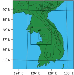
Figure 1. The 850 hPa wind (m s−1, arrows), geopotential height (m, contours), and equivalent potential temperature (K, shaded) at 21:00 LST on 26 July 2011 over northeastern Asia. The rectangle on the Korean Peninsula marks Domain 3, which is explained in Sect. 3.2 and shown in Fig. 2.

2 Case description

The MCS was observed in the Seoul area, South Korea, over a period between 09:00 LST (local solar time) 27 July and 09:00 LST 28 July 2011. A significant amount of precipita-tion is recorded during this period, with a local maximum value of ∼ 200.0 mm h−1. This heavy rainfall caused flash floods and landslides, leading to the deaths of 60 people (Korea Meteorological Administration, 2011). At 21:00 LST 26 July 2011, favorable synoptic-scale features for the de-velopment of the selected MCS and heavy rainfall were ob-served. The western Pacific subtropical high (WPSH) was located over the southeast of South Korea and Japan, and there was a low-pressure trough over north China (Fig. 1). Low-level jets between the flank of the WPSH and the low-pressure system brought warm, moist air from the Yellow Sea to the Korean Peninsula (Fig. 1). Transport of warm and moist air by the southwesterly low-level jet is an impor-tant condition for the development of heavy rainfall events over the Korean Peninsula (Hwang and Lee, 1993; Lee et al., 1998; Seo et al., 2013).

3 CSRM and simulations 3.1 CSRM

As a CSRM, we use the Advanced Research Weather Re-search and Forecasting (ARW) model (version 3.3.1), which

35 ̊ N 36 ̊ N 37 ̊ N 38 ̊ N 39 ̊ N 40 ̊ N 124 ̊ E 126 ̊ E 128 ̊ E 130 ̊ E d03 d02

Figure 2. Triple-nested domains used in the CSRM simulations. The boundary of the figure itself is that of Domain 1, while the rectangles marked by “d02” and “d03” represent the boundary of Domain 2 and Domain 3, respectively. The dotted line represents the boundary of Seoul and terrain heights are contoured every 250 m.

is a nonhydrostatic compressible model. Prognostic micro-physical variables are transported with a fifth-order mono-tonic advection scheme (Wang et al., 2009). Shortwave and longwave radiation parameterizations have been included in all simulations by adopting the Rapid Radiation Transfer Model (RRTM; Mlawer et al., 1997; Fouquart and Bonnel, 1980). The effective sizes of hydrometeors are calculated in a microphysics scheme that is adopted by this study and the calculated sizes are transferred to the RRTM. Then, the ef-fects of the effective sizes of hydrometeors on radiation are calculated in the RRTM.

To represent microphysical processes, the CSRM employs a bin scheme. The bin scheme employed is based on the He-brew University Cloud Model (HUCM) described by Khain et al. (2011). The bin scheme solves a system of kinetic equa-tions for size distribution funcequa-tions for water drops, ice crys-tals (plate, columnar, and branch types), snow aggregates, graupel, hail, and cloud condensation nuclei (CCN). Each size distribution is represented by 33 mass doubling bins, i.e., the mass of a particle mk in the k bin is determined as

mk=2mk−1.

3.2 Control run

For a three-dimensional simulation of the observed MCS, i.e., the control run, two-way interactive triple-nested do-mains with a Lambert conformal map projection as shown in Fig. 2 are adopted. A domain with a 500 m resolution cov-ering the Seoul area (Domain 3) is nested in a domain with a 1.5 km resolution (Domain 2), which in turn is nested in

a domain with a 4.5 km resolution (Domain 1). The length of Domain 3 in the east–west direction is 220 km, while the length in the north–south direction is 180 km. The lengths of Domain 2 and Domain 3 in the east–west direction are 390 and 990 km, respectively, and those in the north–south direction are 350 and 1100 km, respectively. The Seoul area is a conurbation area that is centered in Seoul and includes Seoul and surrounding highly populated cities. Hence, the Seoul area is composed of multiple cities whose total popu-lation is ∼ 25 million. The boundary of Seoul, which has the largest population among those cities, is marked by a dot-ted line in Fig. 2. Black contours in Fig. 2 represent terrain heights. They indicate that most high terrain is located on the eastern part of the Korean Peninsula and the Seoul area is not affected by high terrain. All domains have 84 vertical layers with a terrain following the sigma coordinate, and the model top is 50 hPa. Note that a cumulus parameterization scheme is used in Domain 1 but not used in Domain 2 and Domain 3 where convective rainfall generation is assumed to be explicitly resolved. Here, we use a cumulus parame-terization scheme that was developed by Kain and Fritsch (1990, 1993). This scheme is shown to work reasonably well for resolutions that are similar to what is used for Domain 1 (Gilliland and Rowe, 2007).

Reanalysis data, which are produced by the Met Office Unified Model (Brown et al., 2012) and recorded continu-ously every 6 h on a 0.11◦×0.11◦grid, provide the initial and boundary conditions of potential temperature, specific humidity, and wind for the simulation. These data represent the synoptic-scale environment. For the control run, we em-ploy an open lateral boundary condition. Using the Noah land surface model (LSM; Chen and Dudhia, 2001), surface heat fluxes are predicted.

The current version of the ARW model assumes horizon-tally homogeneous aerosol properties. For the control run that focuses on the effect of aerosol on torrential rain in an urban area (i.e., Seoul area) where aerosol properties such as composition and number concentration vary significantly in terms of time and space, we abandon this assumption of homogeneity and consider the spatiotemporal variability in aerosol properties over the urban area. For this, we develop an aerosol preprocessor that is able to represent the vari-ability in aerosol properties. This aerosol preprocessor in-terpolates observed background aerosol properties such as aerosol mass (e.g., PM10) at observation sites to model grid

points and time steps. This aerosol preprocessor is now im-plemented in the ARW model.

The variability in aerosol properties is observed by sur-face sites that measure PM10 in the Seoul area. These sites

are distributed with about 1 km distance between them and measure aerosol mass every ∼ 10 min, which enables us to resolve the variability with high spatiotemporal resolutions. However, the measurement of other aerosol properties such as aerosol composition and size distributions at those sites is absent. There are additional sites of the AErosol RObotic

10-2 ₁₀₁₀-1-1 ₁₀0 ₁₀₁₀1 100 107 D (diameter, m) dN / d lnD ( cm -3 ₎ µ

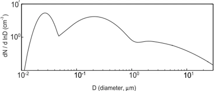
Figure 3. Aerosol size distribution at the surface. N represents aerosol number concentration per unit volume of air and D rep-resents aerosol diameter.

NETwork (AERONET; Holben et al., 2001) in the Seoul area. Distances between these AERONET sites are ∼ 10 km; hence, they do not provide data whose resolutions are as high as those of the PM10 data. However, the AERONET sites

provide information on aerosol composition and size dis-tributions. While using data from the high-resolution PM10

sites to represent the variability in aerosol properties over the Seoul area, we use the relatively low-resolution data from the AERONET sites to represent aerosol composition and size distributions.

AERONET measurements indicate that overall, aerosol particles in the Seoul area during the MCS period follow a trimodal lognormal distribution and aerosol particles, on av-erage, are an internal mixture of 60 % ammonium sulfate and 40 % organic compound. This organic compound is assumed to be water soluble and composed of (by mass) 18 % levoglu-cosan (C6H10O5, density = 1600 kg m−3, van ’t Hoff factor

=1), 41 % succinic acid (C6O4H6, density = 1572 kg m−3,

van ’t Hoff factor = 3), and 41 % fulvic acid (C33H32O19,

density = 1500 kg m−3, van ’t Hoff factor = 5) based on a simplification of observed chemical composition. This mix-ture is adopted to represent aerosol chemical composition in this study. In this study, aerosol–radiation interactions, which are the effect of aerosol on radiation via the reflection, scattering, and absorption of shortwave and longwave radia-tion by aerosol before its activaradia-tion, are not considered. This is partially motivated by the fact that the mixture includes chemical components that absorb solar radiation insignifi-cantly compared to strong radiation absorbers such as black carbon. Based on the AERONET observation, in this study, the trimodal lognormal distribution is assumed for the size distribution of background aerosol as exemplified in Fig. 3. Stated differently, it is assumed that the size distribution of background aerosol at all grid points and time steps has size distribution parameters or the shape of distribution that is identical to that in Fig. 3. The assumed shape of the size dis-tribution of background aerosol is obtained by averaging size distribution parameters (i.e., modal radius and standard devi-ation of nuclei, accumuldevi-ation, and coarse modes each, and the partition of aerosol number among those modes) over the

AERONET sites and the MCS period. With these assump-tion and adopassump-tion, PM10 is converted to background aerosol

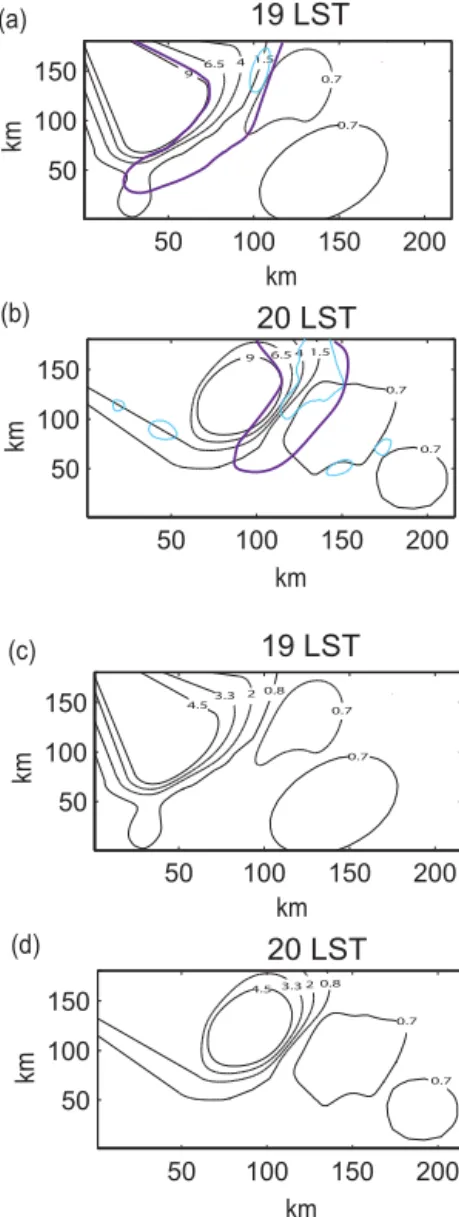
number concentrations. Figure 4a and b show example spa-tial distributions of background aerosol number concentra-tions at the surface in Domain 3 (which covers the Seoul area), which are applied to the control run and represented by black contours. These distributions in Fig. 4a and b are cal-culated based on the surface observation in Domain 3. Blue contours in Fig. 4a and b surround areas with observed heavy precipitation on which this study focuses. In this study, when a precipitation rate at the surface is 60 mm h−1 or above, precipitation is considered heavy precipitation. There is no one universal designated rate (of precipitation) above which precipitation is considered heavy precipitation and the des-ignated rate varies among countries. As a precipitation rate, 60 mm h−1 is around the upper end of the variation. Those blue contours are further discussed in Sect. 4. Purple lines in Fig. 4a and b mark the eastern part of where there is sub-stantial transition from high-value aerosol concentrations to low-value aerosol concentrations. In this transition part, there is reduction in aerosol concentrations by more than a factor of 10 from ∼ 9000 to ∼ 700 cm−3.

In clouds, aerosol size distributions evolve with sinks and sources, which include advection and droplet nucleation (Fan et al., 2009). Aerosol activation is calculated according to the Köhler theory, i.e., aerosol particles with radii exceed-ing a critical value at a grid point are activated to become droplets based on predicted supersaturation, and the corre-sponding bins of the aerosol spectra are emptied. After ac-tivation, aerosol mass is transported within hydrometeors by collision–coalescence and removed from the atmosphere once hydrometeors that contain aerosols reach the surface. It is assumed that in the planetary boundary layer (PBL), back-ground aerosol concentrations do not vary with height but above the PBL background aerosol concentrations reduce ex-ponentially with height. It is also assumed that in non-cloudy areas, aerosol size and spatial distributions are set to fol-low background counterparts. In other words, once clouds disappear completely at any grid point, aerosol size distri-butions and number concentrations at those points recover to background counterparts. This assumption has been used by numerous CSRM studies and proven to simulate overall aerosol properties and their impacts on clouds and precipita-tion reasonably well (Morrison and Grabowski, 2011; Lebo and Morrison, 2014; Lee et al., 2016). This assumption indi-cates that we do not consider the effects of clouds and asso-ciated convective and turbulent mixing on the properties of background aerosol. Also, the prescription of those proper-ties (e.g., number concentration, size distribution, and chem-ical composition) explained above indicates that this study does not take aerosol physical and chemical processes into account. This enables the confident isolation of the sole ef-fects of given background aerosol on clouds and precipita-tion in the Seoul area, which has not been understood well,

50 100 150 200 50 100 150 50 100 150 200 50 100 150 km km (a) (b) km km 9 6.5 4 1.5 _0.7 0.7 9 6.5 4 1.5 0.7 0.7 19 LST 20 LST 50 100 150 200 50 100 150 50 100 150 200 50 100 150 km km (c) (d) km km 4.53.3 2 0.8 0.7 0.7 4.5 3.3 2 0.8 0.7 0.7 19 LST 20 LST

Figure 4. Spatial distributions of background aerosol number con-centrations at the surface (black contours; in ×103cm−3) and the boundary of each area that has a precipitation rate of 60 mm h−1or above (blue contours) in Domain 3 at (a) 19:00 and (b) 20:00 LST. Purple lines in panels (a) and (b) mark a part of the domain in which there is a substantial reduction in aerosol number concentrations (see text for the details of purple lines). Panels (c) and (d) are the same as panels (a) and (b), respectively, but with reduced contrast in aerosol number concentrations for the low-aerosol run (see text for the details of reduced contrast).

by excluding those aerosol processes and cloud effects on background aerosol.

3.3 Additional runs

As seen in Fig. 4a and b at 19:00 and 20:00 LST 27 July 2011, there is a large variability in background aerosol concentrations in the Seoul area. This variability is generated by contrast between the high aerosol concentra-tions in the western part of the domain where aerosol

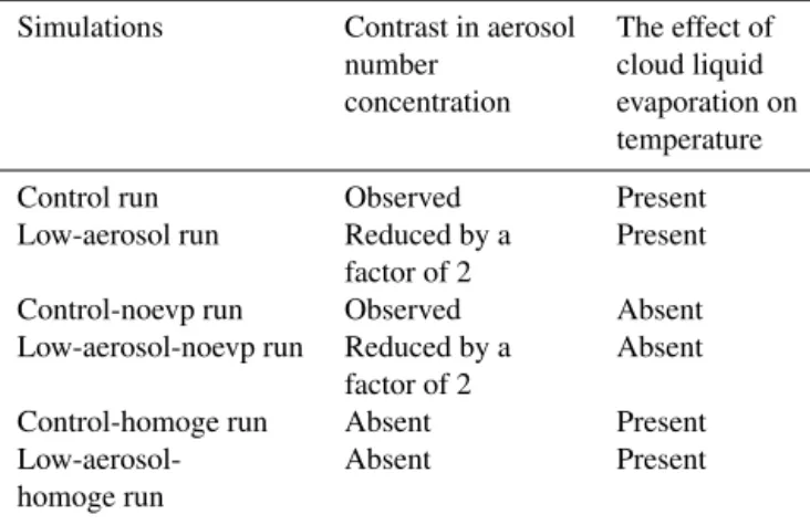
concen-Table 1. Summary of simulations.

Simulations Contrast in aerosol The effect of

number cloud liquid

concentration evaporation on temperature

Control run Observed Present

Low-aerosol run Reduced by a Present

factor of 2

Control-noevp run Observed Absent

Low-aerosol-noevp run Reduced by a Absent factor of 2

Control-homoge run Absent Present

Low-aerosol- Absent Present

homoge run

tration is greater than 1500 cm−3, and the low aerosol con-centrations in the eastern part of the domain where aerosol concentration is ∼ 700 cm−3 or less. As mentioned above, this study focuses on the effect of the spatial variability and loading (or concentrations) of aerosol on precipitation. To better identify and elucidate the effect, the control run is re-peated but with the abovementioned contrast that is reduced. To reduce contrast, over the whole simulation period, the concentrations of background aerosol in the western part of the domain are reduced by a factor of 2, while those in the eastern part do not change. This means that the reduction in the variability accompanies that in aerosol concentrations, which enables us to examine both the effects of the vari-ability and those of concentrations. Note that high and low aerosol concentrations on the left (or western) side and the right (or eastern) side of the domain, respectively, are main-tained throughout the whole simulation period, although the location of the boundary between those sides changes with time. Here, in the process of the reduction in contrast, no changes are made for aerosol chemical compositions and size distributions in both parts of the domain. As examples, the spatial distribution of background aerosol concentrations at the surface with reduced contrast at 19:00 and 20:00 LST 27 July 2011 is shown in Fig. 4c and d, respectively. With reduced contrast and concentrations, the variability and con-centrations of aerosol are lower in this repeated run than in the control run. The repeated simulation has low variability and concentrations of aerosol as compared to the control run and thus is referred to as the “low-aerosol” run. Comparisons between the control run and the low-aerosol run give us a chance to better understand roles played by the spatial vari-ability and loading of aerosol in the spatial distribution of precipitation, which involves torrential rain.

In addition to the control run and the low-aerosol run, there are more simulations that are performed to better understand the effect of aerosol on precipitation here. To isolate the ef-fects of aerosol concentrations on precipitation from those of aerosol spatial variability or vice versa, the control run and

the low-aerosol run are repeated with homogeneous spatial distributions of aerosol. These homogeneous spatial distri-butions mean that there is no contrast in aerosol number con-centrations between the western part of the domain and the eastern part, and aerosol number concentrations do not vary over the domain. The repeated simulations are referred to as the “control-homoge” run and the “low-aerosol-homoge” run. The analyses of model results below indicate that dif-ferences in precipitation between the control run and the low-aerosol run are closely linked to cloud liquid evapora-tive cooling and to elucidate this linkage, the control run and the low-aerosol run are repeated again by turning off cool-ing from cloud liquid evaporation. These repeated simula-tions are referred to as the “control-noevp” run and the “low-aerosol-noevp” run. While a detailed description of those re-peated simulations is given in Sect. 4.3, a brief description is given in Table 1.

4 Results

In this study, analyses of results are performed only in the Seoul area (or Domain 3) where the 500 m resolution is ap-plied. Hence, in the following, the description of the simula-tion results and their analyses is only over Domain 3, unless otherwise stated.

4.1 Meteorological fields, microphysics, and precipitation

4.1.1 Meteorological fields and cumulative precipitation

Figure 5 shows the observed and simulated vertical pro-files of potential temperature, water vapor mass density, u-wind speed, and v-u-wind speed, which represent meteorolog-ical fields. Radiosonde data as observation data are averaged over observation sites in the domain and the simulation pe-riod, while simulated meteorological fields are averaged over the domain and the simulation period to obtain the profiles. Positive (negative) u-wind speed represents eastward (west-ward) wind speed, while positive (negative) v-wind speed represents northward (southward) wind speed. Comparisons between the observed profiles and the simulated counter-parts show that overall differences between them are within ∼10 % of observed values. Hence, with confidence, it can be considered that the simulation of meteorological fields is performed reasonably well.

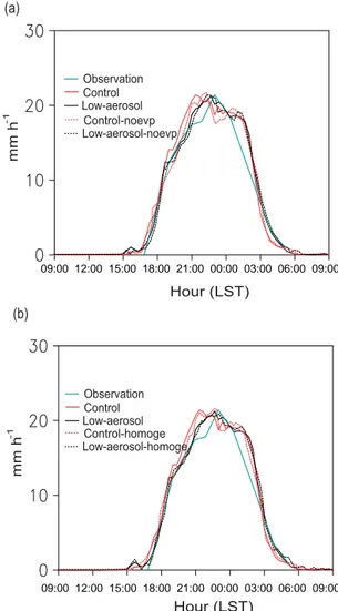
The area-mean precipitation rate at the surface smoothed over 3 h for the control run and the low-aerosol run is de-picted by solid lines in Fig. 6. Dotted lines in Fig. 6 depict the precipitation rate for the repeated control run and low-aerosol run and will be discussed in Sect. 4.3. The simulated precip-itation rate in the control run follows the observed counter-part well, which demonstrates that simulations perform rea-sonably well. Here, observed precipitation is obtained from

4 8 12 16 0 280 300 320 340 360 Potential temperature (K) Height (km) Observation Simulation 4 8 12 16 0 Height (km) Observation Simulation 3 6 9 12 15 18 21 24 m s-1 u-wind speed ( ) 4 8 12 16 0 Height (km) (a) 4 8 12 16 0 0 5 10 15 20 Observation Simulation g m Height (km) -3 Water vapor mass density ( )

(b) (c) -10 -5 0 5 10 15 20 (d) m s-1 v-wind speed ( ) Observation Simulation

Figure 5. Vertical distributions of the averaged (a) potential tem-perature, (b) water vapor mass density, (c) u-wind speed, and (d) v-wind speed. Positive (negative) u-v-wind speed represents eastward (westward) wind speed, while positive (negative) v-wind speed rep-resents northward (southward) wind speed. Observations are aver-aged over observation sites in Domain 3 and the simulation period, while simulations are averaged over Domain 3 and the simulation period. Observation Control mm h -1 Hour (LST) Low-aerosol Observation Control mm h -1 Hour (LST) Low-aerosol Control-homoge Low-aerosol-homoge Control-noevp Low-aerosol-noevp (a) (b) 09:00 12:00 15:00 18:00 21:00 00:00 03:00 06:00 09:00 09:00 12:00 15:00 18:00 21:00 00:00 03:00 06:00 09:00

Figure 6. Time series of the area-mean precipitation rates at the surface smoothed over 3 h for the control run, the low-aerosol run, and observations in Domain 3. In panel (a), the rates in the control-noevp run and the low-aerosol-control-noevp are additionally shown, while in panel (b), the rates in the control-homoge run and the low-aerosol-homoge are additionally shown.

measurement by rain gauges that are parts of the automatic weather station (AWS) at the surface. The AWS has a spa-tial resolution of ∼ 3 km. Also, the temporal evolution of the mean precipitation rate in the control run is very similar to that in the low-aerosol run. Associated with this similarity, the averaged cumulative precipitation over the domain at the last time step for the control run is 154.7 mm, which is just ∼3 % greater than 150.2 mm for the low-aerosol run. 4.1.2 Precipitation fields and frequency distributions Figure 7a, b, and c show frequency distributions of precipi-tation rates that are collected over all time steps and all grid points at the surface in the simulations. In Fig. 7, solid lines represent frequency distributions for the control run and the low-aerosol run, while dashed lines represent those for the

Low-aerosolControl 100 101 102 103 104 105 106 Precipitation frequency 50 100 150 200 0 (b) 100 101 102 103 104 105 106 Precipitation frequency 50 100 150 200 0 (g) Low-aerosolControl 50 100 150 200 0 100 101 102 103 104 105 106 Precipitation frequency (d) Low-aerosolControl 100 101 102 103 104 105 106 Precipitation frequency 50 100 150 200 0 (j) Low-aerosolControl 0 50 100 150 200 100 101 102 103 104 105 106 Precipitation frequency (m) Low-aerosolControl Whole period 17:00–19:00 LST Observation 50 100 150 200 0 100 101 102 103 104 105 106 Precipitation frequency (e) Low-aerosolControl 100 101 102 103 104 105 106 Precipitation frequency 50 100 150 200 0 (h) Low-aerosolControl 0 50 100 150 200 100 101 102 103 104 105 106 Precipitation frequency (n) Low-aerosolControl Low-aerosolControl 100 101 102 103 104 105 106 Precipitation frequency 50 100 150 200 0 Precipitation rate (mm h ) -1

(a) Whole period Observation Low-aerosol-noevpControl-noevp 100 101 102 103 104 105 106 Precipitation frequency 50 100 150 200 0 (k) Low-aerosolControl 50 100 150 200 0 100 101 102 103 104 105 106 Precipitation frequency (f) Low-aerosolControl 100 101 102 103 104 105 106 Precipitation frequency 50 100 150 200 0 (i) 100 101 102 103 104 105 106 Precipitation frequency 50 100 150 200 0 (l) 0 50 100 150 200 100 101 102 103 104 105 106 Precipitation frequency (o) Low-aerosolControl 100 101 102 103 104 105 106 Precipitation frequency 50 100 150 200 0 (c) Whole period Observation Control-noevp Low-aerosol-noevp Control-noevp Low-aerosol-noevp Control-noevp Low-aerosol-noevp Low-aerosol-noevpControl-noevp Control-homoge Low-aerosol-homoge Control-homoge Low-aerosol-homoge Low-aerosolControl Control-homoge Low-aerosol-homoge Low-aerosolControl Control-homoge Low-aerosol-homoge Low-aerosolControl Control-homoge Low-aerosol-homoge Precipitation rate (mm h ) -1 _{Precipitation rate (mm h )} -1

Precipitation rate (mm h ) -1 _{Precipitation rate (mm h )} -1 _{Precipitation rate (mm h )} -1

Precipitation rate (mm h ) -1 _{Precipitation rate (mm h )} -1 _{Precipitation rate (mm h )} -1

Precipitation rate (mm h ) -1 _{Precipitation rate (mm h )} -1 _{Precipitation rate (mm h )} -1

Precipitation rate (mm h ) -1 _{Precipitation rate (mm h )} -1 _{Precipitation rate (mm h )} -1

17:00–19:00 LST 17:00–19:00 LST

19:00–20:00 LST 19:00–20:00 LST 19:00–20:00 LST

20:00–23:00 LST 20:00–23:00 LST 20:00–23:00 LST

04:00–05:00 LST 04:00–05:00 LST 04:00–05:00 LST

Figure 7. Frequency distributions of the precipitation rates at the surface, which are collected over the whole domain, for (a, b, c) the whole simulation period, (d, e, f) a period between 17:00 and 19:00 LST, (g, h, i) a period between 19:00 and 20:00 LST, (j, k, l) a period between 20:00 and 23:00 LST, and (m, n, o) a period between 04:00 and 05:00 LST. In panels (a), (b), and (c) observed frequency, which is interpolated to the simulation time steps and grid points, is also shown.

repeated control run and low-aerosol run, which will be de-scribed in Sect. 4.3. Figure 7a, d, g, j, and m show frequency distributions only for the control run and the low-aerosol run. The other panels in Fig. 7 are supposed to show distribu-tions only for the repeated control run and low aerosol run; however, for comparisons among the control run, the low-aerosol run, and the repeated runs, the control run and the low-aerosol run are displayed as well in those panels.

In Fig. 7a, b, and c, frequency distributions of observed precipitation rates that are interpolated to grid points and time steps in the simulations are also shown. The observed maximum precipitation rate is ∼ 180 mm h−1, which is sim-ilar to that in the control run. Also, observed frequency distribution is consistent with the simulated counterpart in the control run, although it appears that particularly for heavy precipitation with rates above 60 mm h−1, the simu-lated frequency is underestimated compared to the observed counterpart. The overall difference in frequency distributions between observation and the control run is much smaller than those between the control run and the low-aerosol run. Hence, we assume that the difference between observation and the control run is considered negligible compared to that among the runs. Based on this, when it comes to a discussion about the difference between the control run and the low-aerosol run, results in the control run can be assumed to be benchmark results against which the effect of decreases in the spatial variability and concentrations of aerosol on results in the low-aerosol run can be assessed.

While we do not see a large difference in cumulative pre-cipitation between the control run (154.7 mm) and the low-aerosol run (150.2 mm), the frequency distribution of precipi-tation rates shows distinctively different features between the control run and the low-aerosol run (Fig. 7a). For precipita-tion with rates above 60 mm h−1or heavy precipitation, cu-mulative frequency is ∼ 60 % higher for the control run. For certain ranges of precipitation rates above 60 mm h−1, there are increases in cumulative frequency by a factor of as much as ∼ 10 to ∼ 100. Moreover, for precipitation rates above 120 mm h−1, while there is the presence of precipitation in the control run, there is no precipitation in the low-aerosol run. Hence, we see that there are significant increases in the frequency of heavy precipitation in the control run compared to that in the low-aerosol run.

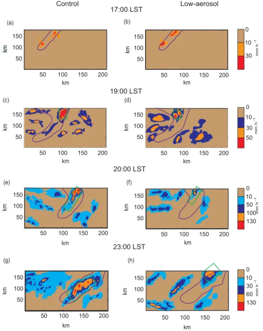
Figure 8 shows spatial distributions of precipitation rates at the surface. Purple lines in Fig. 8 mark the eastern part of where there is substantial transition from high-value aerosol concentrations to low-value aerosol concentrations as in Fig. 4. In this transition part, as explained in Fig. 4, there is reduction in aerosol concentrations by more than a factor of 10. Figure 8a and b show those distributions at 17:00 LST 27 July 2011 corresponding to initial stages of the precip-itating system in the control run and the low-aerosol run, respectively. At 17:00 LST, there is a small area of precip-itation around the northwest corner of the domain in both the control run and the low-aerosol run. This implies that a

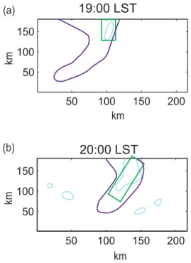
small cloud system develops around the northwest corner of the domain at 17:00 LST. The size of the system and its pre-cipitation area grow with time and at 19:00 LST, the size is much larger (Fig. 8c and d). The maximum precipitation rate reaches ∼ 100 mm h−1when time progresses to 19:00 LST (Fig. 7d). Heavy precipitation is concentrated in a specific area (surrounded by the green rectangle) in both of the runs (Fig. 8c and d). The green rectangle surrounds a specific area where more than 90 % of the events of heavy precipitation (over the domain) with rates above 60 mm h−1occur in each of the runs at 19:00 LST. Since heavy precipitation starts to form around 19:00 LST, the green rectangle starts to be iden-tified around 19:00 LST. Contrast in precipitation between the green rectangle and the other areas in the domain gen-erates an inhomogeneity in the spatial distribution of precip-itation. The location of the specific area in the control run is consistent with the location of heavy precipitation in ob-servation as seen in comparisons between Figs. 4a, 8c, and 9a. Figure 9a shows the blue contour, which surrounds areas with observed heavy precipitation in Fig. 4a, and the green rectangle, which surrounds the specific area where more than 90 % of the events of heavy precipitation occur in Fig. 8c. In Fig. 9a, the purple line, which marks a substantial transition in aerosol concentrations in Fig. 4a, is also shown. The good consistency among the locations demonstrates that the simu-lation of the spatial distribution of heavy precipitation is per-formed reasonably well. Between 17:00 and 19:00 LST, we do not see significant differences in the frequency distribu-tion of precipitadistribu-tion rates, particularly in heavy precipitadistribu-tion with rates above 60 mm h−1between the control run and the low-aerosol run (Fig. 7d).

By 20:00 LST, the maximum rate of torrential rain reaches ∼130 mm h−1 for the control run and ∼ 110 mm h−1 for the low-aerosol run (Fig. 7g). Associated with this, between 19:00 and 20:00 LST, significant differences in frequency distributions, particularly for heavy precipitation between the control run and the low-aerosol run, start to appear (Fig. 7g). At 20:00 LST as seen in Fig. 8e and in the previous hours, in the control run more than 90 % of heavy precipitation events are concentrated in a specific area that is surrounded by the green rectangle. Note that only in this specific area, does ex-tremely heavy precipitation with rates above 100 mm h−1 oc-cur. In the low-aerosol run, the extremely heavy precipita-tion with rates above 100 mm h−1also occurs only in a par-ticular area, which is surrounded by the green rectangle, at 20:00 LST (Fig. 8f). At 20:00 LST, as seen in Fig. 4b, obser-vation shows that there are five spots of heavy precipitation. The location of the largest spot where most heavy precipi-tation events occur is similar to that of the specific area that is surrounded by the green rectangle in the control run as seen in comparisons between Figs. 4b, 8e, and 9b. Figure 9b shows the blue contour and the purple line from Fig. 4b and the green rectangle from Fig. 8e. This again demonstrates that the simulation of the spatial distribution of heavy pre-cipitation is performed with fairly good confidence.

50 100 150 200 50 100 150 kmkm km (a) (b) 17:00 LST Control Low-aerosol 50 100 150 200 50 100 150 km km 50 100 150 200 50 100 150 km km (c) (d) 50 100 150 200 50 100 150 50 100 150 200 50 100 150 km km km km (e) (f) 20:00 LST 50 100 150 200 50 100 150 km km 50 100 150 km 50 100 150 200 km (g) (h) 23:00 LST 50 100 150 200 50 100 150 km km 19:00 LST km 0 10 30 0 10 30 50 0 10 50 100 130 0 10 30 60 130 mm h -1 mm h -1 mm h -1 mm h -1

Figure 8. Spatial distributions of precipitation rates at the surface. Green rectangles mark areas with heavy precipitation and are described in detail in text. Purple lines mark the eastern part of where there is substantial transition from high-value aerosol concentrations to low-value aerosol concentrations as in Fig. 4. Panels (a), (c), (e), and (g) are for the control run, while panels (b), (d), (f), and (h) are for the low-aerosol run. Panels (a) and (b) are for 17:00 LST, and panels (c) and (d) are for 19:00 LST. Panels (e) and (f) are for 20:00 LST, and panels (g) and (h) are for 23:00 LST.

The system propagates eastwards after 20:00 LST in a way that its easternmost part is closer to the east boundary of the domain as seen in comparisons between Fig. 8e (Fig. 8f) and Fig. 8g (Fig. 8h) for the control (low-aerosol) run. As seen in Fig. 8g and in the previous hours, for the control run more than 90 % of heavy precipitation events are concen-trated in a specific area (surrounded by the green rectangle) at 23:00 LST. However, in the low-aerosol run, heavy pre-cipitation is not concentrated in a specific area at 23:00 LST. Unlike the green rectangle in the control run at 23:00 LST, the green rectangle at 23:00 LST in the low-aerosol run

sur-rounds an area where ∼ 50 % of heavy precipitation events are located, although the rectangle surrounds the largest area with heavy precipitation among heavy precipitation areas in the low-aerosol run. For a period between 20:00 and 23:00 LST compared to that between 19:00 and 20:00 LST, the maximum precipitation rate rises up to ∼ 180 mm h−1in the control run; however, in the low-aerosol run, the maxi-mum precipitation rate stays at ∼ 120 mm h−1(Fig. 7g and j). Hence, there is the presence of precipitation rates between ∼120 and ∼ 180 mm h−1in the control run, while there is their absence in the low-aerosol run for the period between

50 100 150 200 50 100 150 km km (a)

19:00 LST

20:00 LST

Figure 9. Boundary of each area which has the observed surface precipitation rate of 60 mm h−1or above (blue contours) and a spe-cific area (surrounded by the green rectangle in the control run and described in the text related to Fig. 8) where heavy precipitation is concentrated in the control run in Domain 3 at (a) 19:00 LST and (b) 20:00 LST. Purple lines are the same as in Fig. 8.

20:00 and 23:00 LST. This reflects that increases in the fre-quency of torrential rain, which are induced by increases in the spatial variability and loading of aerosol, enhance as the system evolves from its initial stage before 20:00 LST to its mature stage between 20:00 and 23:00 LST.

Of interest is that the green rectangle is included in an area which is surrounded by the purple line in all panels with different times in Fig. 8 and further discussion for this mat-ter is provided in Sect. 4.2. Afmat-ter 23:00 LST 27 July 2011, the precipitating system enters its decaying stage. Figure 7m shows precipitation-rate frequency in the control run and the low-aerosol run for a period between 04:00 and 05:00 LST 28 July 2011. As seen in Fig. 7m, with the progress of the de-caying stage, the maximum precipitation rate reduces down to ∼ 25 mm h−1as an indication that heavy precipitation dis-appears and the system is nearly at the end of its life cycle. 4.2 Dynamics

Convergence

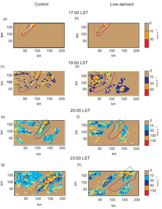
For the examination of condensation which is the main source of precipitation, convergence fields at the surface, where updrafts that produce condensation originate, are ob-tained and the column-averaged condensation rates are su-perimposed on them. Other processes such as deposition and freezing produce the mass of solid hydrometeors and act as

sources of precipitation; however, their contribution to pre-cipitation is ∼ 1 order of magnitude smaller than that by con-densation in the control run and the low-aerosol run. Hence, here, among sources of precipitation, we focus on condensa-tion. Convergence and condensation fields are again superim-posed on shaded precipitation fields as shown in Fig. 10. In Fig. 10, convergence and condensation fields are represented by white and yellow contours, respectively. When it comes to the convergence field in the green rectangle in Fig. 10, which starts to be formed around 19:00 LST and is composed of convergence lines, the field in the rectangle in the control run is stronger than that in the low-aerosol run. The averaged in-tensity of the convergence field over an area with non-zero convergence in the green rectangle and over the simulation period is 0.013 s−1 in the control run, while the averaged intensity is 0.007 s−1 in the low-aerosol run. The conver-gence field in the green rectangle is strongest among con-vergence lines over the whole domain and, associated with this, stronger updrafts and greater condensation develop over that field in the green rectangle than in the other lines over the whole domain in each of the runs.

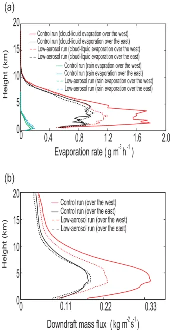
Figure 11 shows horizontal distributions of wind vector field (arrows) superimposed upon fields of convergence, con-densation, and precipitation. In general, particularly from 19:00 LST on, in the area with high-value aerosol concentra-tions to the west of the strong convergence field (surrounded by the green rectangle), there are greater horizontal wind speeds than in the area with low-value aerosol concentra-tions to the east of the strong convergence field in the con-trol run. As seen in comparisons between the location of the rectangle and that of the purple line, which mark the tran-sition zone for aerosol concentrations, the area to the west of the rectangle has higher aerosol concentrations than that to the east. In the area with high-value aerosol concentra-tions, there is greater cloud liquid evaporation occurring than in the area with low-value aerosol concentrations in the con-trol run as shown in Fig. 12a. Figure 12a shows the vertical distribution of the time- and domain-averaged cloud liquid and rain evaporation rates over each of the areas to the west and east of the strong convergence field, which is surrounded by the green rectangle, and over the period between 17:00 and 19:00 LST for the control run and the low-aerosol run. For the calculation of the averaged values in Fig. 12, the area to the west (east) of the strong convergence field is set to include all parts of the north–south direction, which is the y direction, and the vertical domains but only a portion of the east–west direction domain, which is the x-direction do-main that extends from the western boundary of Dodo-main 3 to 90 km where the western boundary of the green rectan-gle at 19:00 LST is located (from 110 km where the eastern boundary of the green rectangle at 19:00 LST is located to the eastern boundary of Domain 3) in Domain 3 for the con-trol run. For the low-aerosol run, the area to the west (east) of the strong convergence field is identical to that in the con-trol run except for the fact that the area includes a portion of

kmkm km (a) (b) Control Low-aerosol 50 100 150 200 50 100 150 km km 50 100 150 200 50 100 150 km km (c) (d) 50 100 150 200 50 100 150 50 100 150 200 50 100 150 km km km km (e) (f) 50 100 150 200 50 100 150 km km 50 100 150 km 50 100 150 200 km (g) (h) 50 100 150 200 50 100 150 km km km 0 10 30 0 10 30 50 0 10 50 100 130 0 10 30 60 130 100 50 100 150 200 50 100 150 17:00 LST 20:00 LST 23:00 LST 19:00 LST mm h -1 mm h -1 mm h -1 mm h -1

Figure 10. Same as Fig. 8 but with convergence at the surface (white contours) and the column-averaged condensation rates (yellow contours) which are superimposed on the precipitation field. In panels (a) and (b), white contours are at 0.4 and 0.7×10−2s−1and yellow contours are at 0.4 and 0.9 g m−3h−1. In panels (c) and (d), white contours are at 0.9 and 1.7×10−2s−1and yellow contours are at 0.9 and 1.5 g m−3h−1. In panels (e) and (f), white contours are at 1.4 and 2.3 × 10−2s−1and yellow contours are at 1.3 and 2.9 g m−3h−1. In panels (g) and (h), white contours are at 2.1 and 3.5 × 10−2s−1and yellow contours are at 2.3 and 3.8 g m−3h−1.

the x-direction domain that extends from the western bound-ary of Domain 3 to 70 km where the western boundbound-ary of the green rectangle at 19:00 LST is located (from 90 km where the eastern boundary of the green rectangle at 19:00 LST is located to the eastern boundary of Domain 3) in Domain 3.

High-value aerosol concentrations reduce autoconversion and in turn increase cloud liquid as a source of evaporation and thus increase cloud liquid evaporation compared to low-value aerosol concentrations. In addition, high-low-value aerosol concentrations produce high-value cloud droplet number concentration and the associated high-value surface areas of

droplets. The surface of droplets is where condensation oc-curs and as shown by Lee et al. (2009) and a recent study by Fan et al. (2018), the high-value surface areas cause higher-value condensation compared to the situation with low-higher-value aerosol concentrations that lead to lower-value condensa-tion. The averaged condensation rate over the abovemen-tioned area to the west (east) of the strong convergence field and over the period between 17:00 and 19:00 LST is 1.28 (0.97) g m−3h−1 in the control run. This further increases cloud liquid (as a source of evaporation) and thus its evapora-tion in the area with high-value aerosol concentraevapora-tions. Also,

kmkm km (a) (b) Control Low-aerosol 50 100 150 200 50 100 150 km km 50 100 150 200 50 100 150 km km (c) (d) 50 100 150 200 50 100 150 50 100 150 200 50 100 150 km km km km (e) (f) 50 100 150 200 50 100 150 km km 50 100 150 km 50 100 150 200 km (g) (h) 50 100 150 200 50 100 150 km km km 0 10 30 0 10 30 50 0 10 50 100 130 0 10 30 60 130 50 100 150 200 50 100 150 10 m s -1 10 m s -1 10 m s -1 10 m s -1 10 m s -1 _{10 m s} -1 10 m s -1 10 m s -1 mm h -1 mm h -1 mm h -1 mm h -1 17:00 LST 20:00 LST 23:00 LST 19:00 LST

Figure 11. Same as in Fig. 10 but with wind vector fields (arrows), which are superimposed on the precipitation, convergence, and conden-sation fields.

with high-value aerosol concentrations, there is an increase in the surface-to-volume ratio of cloud droplets and this in-creases evaporation efficiency and thus cloud liquid evapo-ration compared to the situation with low-value aerosol con-centrations. However, mainly due to an increase in the size of raindrops and their associated decrease in the surface-to-volume ratio, which is induced by high-value aerosol con-centrations, rain evaporation reduces compared to the situ-ation with low-value aerosol concentrsitu-ations as also shown in van den Heever et al. (2011). Increases in cloud liquid evaporation in turn enhance negative buoyancy, which in-duces stronger downdrafts in the area with high-value aerosol concentrations than in the area with low-value aerosol con-centrations in the control run particularly between 17:00

and 19:00 LST as seen in Fig. 12b. Sublimation and melt-ing also enhance negative buoyancy; however, their contri-bution is ∼ 1 order of magnitude smaller than the contribu-tion by cloud liquid evaporacontribu-tion. Hence, here, we focus on cloud liquid evaporation. Figure 12b shows the vertical dis-tribution of the time- and domain-averaged downdraft mass fluxes over each of the areas to the west and east of the strong convergence field (surrounded by the green rectangle) for the control run and the low-aerosol run over the period between 17:00 and 19:00 LST. Previous studies have shown that aerosol-induced increases in cloud liquid evaporation are closely linked to the enhancement of the intensity of down-drafts (Lee et al., 2008a, b, 2013; Lee, 2017). Cloud liquid or droplets in downdrafts move together with downdrafts; thus,

00

5

10

15

20

0.4

0.8

1.2

1.6

2.0

g m

h

Evaporation rate ( )

Control run (cloud-liquid evapration over the west) Control run (cloud-liquid evaporation over the east) Low-aerosol run (cloud-liquid evaporation over the west) Low-aerosol run (cloud-liquid evaporation over the east)

00

5

10

15

20

0.11

0.22

0.33

Downdraft mass flux (

kg m

)

s

(a)

(b)

Control run (over the west)

Control run (over the east)

Low-aerosol run (over the west)

Low-aerosol run (over the east)

Control run (rain evapration over the west) Control run (rain evaporation over the east) Low-aerosol run (rain evaporation over the west) Low-aerosol run (rain evaporation over the east)

Figure 12. Vertical distributions of the time- and domain-averaged (a) cloud liquid and rain evaporation rates and (b) down-draft mass fluxes over each of the areas to the west and east of the strong convergence field for the control run and the low-aerosol run over a period between 17:00 and 19:00 LST (see text for details).

when downdrafts descend, cloud liquid descends while be-ing included in downdrafts. Cloud liquid in the descendbe-ing downdrafts evaporates. More evaporation of cloud liquid pro-vides greater negative buoyancy to downdrafts so that they accelerate more (Byers and Braham, 1949; Grenci and Nese, 2001).

After reaching the near-surface altitudes below ∼ 3 km, in the control run, stronger downdrafts spread out as stronger outflow or horizontal movement, as seen in the area with high-value aerosol concentrations, compared to those in the area with low-value aerosol concentrations around

19:00 LST in Fig. 11c. The outflow in the area with high-value aerosol concentrations accelerates, due to evaporation on its path, as it moves southeastwards from the northern and western boundaries of the domain. The outflow accel-erates until it collides with surrounding air that has weaker horizontal movement in the area with low-value aerosol con-centrations. This collision mainly occurs in the places where the transition between high-value aerosol concentrations and low-value aerosol concentrations is located (surrounded by the purple line) as seen in Fig. 11c. This collision creates the strong convergence field around 19:00 LST, which is sur-rounded by the green rectangle in those places in the control run as seen in Fig. 11c. Hence, most of the strong conver-gence field (surrounded by the green rectangle) is included in the transition zone between high-value and low-value aerosol concentrations (which is surrounded by the purple line) in the control run (Fig. 11c). The strong convergence field in the green rectangle generates a large amount of condensation and cloud liquid and this large amount of cloud liquid produces not only heavy precipitation but also high-degree of evapo-ration. Then, high-degree of evaporation in turn contributes to the occurrence of a stronger convergence field in the green rectangle, which establishes feedbacks between the conver-gence field, condensation, heavy precipitation, and evapora-tion. This enables the intensification of downdrafts and hor-izontal wind to the west of the convergence field shown in the green rectangle, the convergence field, and the increases in heavy precipitation with time, while the convergence field shown in the green rectangle is advected eastwards in the control run as seen in Figs. 7g, j and 11e and g. As seen in Fig. 11e and g, even after 19:00 LST, the convergence field shown in the green rectangle stays within the transition zone between the high-value and low-value aerosol concentrations (which is surrounded by the purple line) during its eastward advection. This indicates that the collision explained above between strong outflow and surrounding weak wind, which is essential for the formation of the convergence field shown in the green rectangle, continuously occurs in the transition zone even after 19:00 LST.

Note that, associated with aerosol concentrations in the western part of the domain, which are 2 times greater in the control run than in the low-aerosol run, there are differences in aerosol concentrations 2 times greater between the area with high-value aerosol concentrations and that with low-value aerosol concentrations in the control run than in the low-aerosol run. This leads to a transition in aerosol con-centrations 2 times greater , particularly in the transition zone surrounded by the purple line in the control run than in the low-aerosol run (Fig. 4). Associated with this, there is a greater reduction in autoconversion and increases in cloud liquid and surface-to-volume ratio of cloud droplets in the area with high-value aerosol concentrations in the control run than in the low-aerosol run. Then, there is greater evapora-tion, intensity of downdrafts, and associated outflow and its acceleration during its southeastward movement around the

surface in that area in the control run than in the low-aerosol run (Figs. 11 and 12). This means that there is stronger col-lision between outflow and the surrounding air in the control run than in the low-aerosol run, and stronger collision forms the strong convergence field (in the green rectangle), which is much more intense in the control run than in the low-aerosol run as seen in Figs. 10 and 11. Over this much more intense convergence field, there is the formation of stronger updrafts that are able to form stronger convection, which is in turn able to produce more events of heavy precipitation in the con-trol run than in the low-aerosol run (Fig. 7). The more intense strong convergence field in the green rectangle establishes stronger feedbacks between the convergence field, condensa-tion, heavy precipitacondensa-tion, and evaporation in the control run than in the low-aerosol run. Hence, differences in intensity of the convergence field shown in the green rectangle and in the heavy precipitation between the runs become greater as time progresses (Figs. 7, 10, and 11).

4.3 Sensitivity tests 4.3.1 Evaporative cooling

It is discussed that cloud liquid evaporative cooling plays an important role in the formation of the strong convergence field where most of heavy precipitation occurs (surrounded by the green rectangle) in the control run. To confirm this role, we repeat the control run and the low-aerosol run with cooling from cloud liquid evaporation turned off and cool-ing from rain evaporation left on. The repeated control run and the low-aerosol run are referred to as the control-noevp run and the low-aerosol-noevp run, respectively. In these re-peated runs, cloud liquid mass reduces due to cloud liquid evaporation, although cloud liquid evaporation does not af-fect temperature.

The temporal evolution of precipitation rates in the control-noevp run and the low-aerosol-noevp run is similar to that in the control run and the low-aerosol run (Fig. 6a). However, due to the absence of cloud liquid evaporative cool-ing, there is no formation of strong outflow and convergence field (as seen in wind field and the green rectangle in the control run and the low-aerosol run) in these repeated runs as shown in Fig. 13a and b. Figure 13a and b show wind vec-tor and convergence fields at the surface over the whole do-main in the control-noevp run and the low-aerosol-noevp run, respectively, at 23:00 LST, which corresponds to the mature stage of the system. Note that the strong convergence field is clearly distinguishable in its intensity and length from any other convergence lines in each of the control run and the low-aerosol run as seen in Figs. 10 and 11. However, there is no field in each of the repeated runs that is distinguish-able in its intensity and length from other lines as seen in Fig. 13a and b. This leads to the situation in which there is no particular convergence field in the control-noevp run that produces many more events of heavy precipitation than in the

low-aerosol-noevp run. As seen in Fig. 7h and k, associated with this, differences in the frequency of heavy precipitation with rates above 60 mm h−1 between the repeated runs are much smaller than those between the control run and the low-aerosol run, particularly for the period between 19:00 and 23:00 LST, although the control-noevp run shows a greater frequency of heavy precipitation than the low-aerosol-noevp run. This results in much smaller differences in heavy precip-itation between the repeated runs than between the control run and the low-aerosol run for the whole simulation period as seen in Fig. 7b. This demonstrates that cloud liquid evapo-rative cooling and its differences between the control run and the low-aerosol run play a key role in many more events of heavy precipitation in the control run than in the low-aerosol run.

4.3.2 Variability in aerosol concentrations

Note that between the control run and the low-aerosol run, there are changes not only in the spatial variability in aerosol concentrations but also in aerosol concentrations. This means that differences between those runs are caused not only by changes in the variability but also by changes in aerosol con-centrations. Although there have been many studies on the effects of changes in aerosol concentrations on heavy pre-cipitation, studies on those effects of changes in the variabil-ity have been rare. Motivated by this, as a preliminary step to the understanding of those effects of changes in the vari-ability, here, we attempt to isolate the effects of changes in the variability on heavy precipitation from those in aerosol concentrations or vice versa. For this purpose, the control run and the low-aerosol run are repeated with homogeneous spatial distributions of background aerosol concentrations. These repeated runs are referred to as the control-homoge run and the low-aerosol-homoge run. In the control-homoge run (low-aerosol-homoge run), aerosol concentrations over the domain are fixed at one value, which is the domain-averaged concentration of the background aerosol in the con-trol run (the low-aerosol run), at each time step. Hence, in the control-homoge run and the low-aerosol-homoge run, the variability (or contrast) in the spatial distribution of aerosol concentrations between the area with high-value aerosol con-centrations and that with low-value aerosol concon-centrations is removed, which achieves homogeneous spatial distributions. The temporal evolution of precipitation rates in the control-homoge run and the low-aerosol-homoge run is simi-lar to that in the control run and the low-aerosol run (Fig. 6b). However, with the homogeneity in the spatial distribution of aerosol concentrations, there is no formation of strong out-flow and thus strong convergence field that is distinguishable from any other convergence lines in the control-homoge run and low-aerosol-homoge run as seen in Fig. 13c and d. Fig-ure 13c and d show wind vector and convergence fields over the whole domain at 23:00 LST in the control-homoge run and the low-aerosol-homoge run, respectively. In the absence

23:00 LST (b) (a) Control-noevp km km 50 100 150 200 50 100 150 km 50 100 150 200 50 100 150 km Low-aerosol-noevp 50 100 150 200 50 100 150 km km (c) Control-homoge 50 100 150 200 50 100 150 km km (d) Low-aerosol-homoge 10 m s -1 10 m s -1 10 m s -1 10 m s -1

Figure 13. Spatial distributions of convergence (red contours) and wind vector (arrows) at the surface at 23:00 LST. Panels (a), (b), (c), and (d) are for the control-noevp run, the low-aerosol-noevp run, the control-homoge run, and the low-aerosol-homoge run, respectively, and contours are at 2.1 and 3.5 × 10−2s−1.

of the variability between the area with high-value aerosol concentrations and that with low-value aerosol concentra-tions, there are no differences in evaporative cooling between those areas and thus there is no strong outflow or conver-gence field which is distinguishable from any other lines.

Comparisons between the control run and the control-homoge run (the low-aerosol run and the low-aerosol-homoge run) isolate the effects of the variability on heavy precipitation from those of aerosol concentrations whose av-eraged value is set at an identical value at each time step in the runs. Due to the absence of the variability in the spa-tial distribution of aerosol concentrations and the associ-ated strong convergence field, the frequency of heavy pre-cipitation in the control-homoge run and in the low-aerosol-homoge run is, on average, just ∼ 18 % and ∼ 13 % of that in the control run and in the low-aerosol run, respectively, for the whole simulation period (Fig. 7c). Hence, the pres-ence of the variability alone (in the abspres-ence of changes in aerosol concentrations) increases the number of the heavy precipitation events by a factor of ∼ 5 or ∼ 10. This pres-ence alone also results in a substantial increase in the maxi-mum precipitation rate in the control run and the low-aerosol run compared to the repeated runs. Between the low-aerosol run and the low-aerosol-homoge run, the increase is from 80 mm h−1 in the low-aerosol-homoge run to 120 mm h−1 in the low-aerosol run, while between the control run and the control-homoge run, the increase is significant and from 90 mm h−1in the control-homoge run to 180 mm h−1in the control run (Fig. 7c). Here, we see that even without the ef-fects of changes in aerosol concentrations, the presence of the variability alone is able to cause significant enhancement of

heavy precipitation in terms of its frequency and maximum value.

Remember that there is an identical domain-averaged background aerosol concentration at each time step between the control run and the control-homoge run and between the low-aerosol run and the low-aerosol-homoge run. Hence, changes in the averaged aerosol concentration between the control-homoge run and the low-aerosol-homoge run are identical to those between the control run and the low-aerosol run. With these identical changes in the averaged aerosol concentration, between the control run and the low-aerosol run, there are additional changes in the variability in aerosol distributions. There is a larger frequency of heavy precip-itation in the control-homoge run than in the low-aerosol-homoge run (Fig. 7c). However, as mentioned above, there is no strong convergence field which is distinguishable from any other lines in the control-homoge run, as seen in Fig. 13c. Associated with this, differences in the frequency of heavy precipitation between the control-homoge run and the low-aerosol-homoge run are much smaller than those between the control run and the low-aerosol run, particularly during the period between 19:00 and 23:00 LST, as seen in Fig. 7i and l. This results in a situation in which differences in the fre-quency of heavy precipitation between the control-homoge run and the low-aerosol-homoge run are, on average, just ∼15 % of those between the control run and the low-aerosol run for the whole simulation period (Fig. 7c). With identi-cal changes in the averaged aerosol concentration between a pair of the control run and the low-aerosol run and a pair of the control-homoge run and the low-aerosol-homoge run, this demonstrates that additional changes in the variability in aerosol distributions play a much more important role in aerosol-induced increases in the occurrence of heavy precip-itation than changes in the averaged aerosol concentrations.

5 Summary and conclusion

This study examines how aerosol affects heavy precipitation in an urban conurbation area. For this examination, a case that involves an MCS and torrential rain over the conurbation area which is centered in Seoul, South Korea, is simulated. This case has large spatial variability in aerosol concentra-tions, which involves high-value aerosol concentrations in the western part of the domain and low-value aerosol con-centrations in the eastern part of the domain.

It is well-known that increases in aerosol concentrations reduce autoconversion and increase cloud liquid as a source of evaporation, which enhances evaporation and associated cooling. Hence, high-value aerosol concentrations in the western part of the domain cause high-value evaporative cooling rates, while low-value aerosol concentrations in the eastern part of the domain cause low-value evaporative cool-ing rates. Greater evaporative coolcool-ing produces greater neg-ative buoyancy and more intense downdrafts in the western