경북대학교 에너지화공전공

Department of Energy Chemical Engineering

Kyungpook National University, Sangju 386, Gajang-dong Sangju 742-711, Korea

Solution Thermodynamics

CHME232-001

Instructor: Prof. Moon Gab Kim E-mail: mg_kim@knu.ac.kr

Chapter 10.

Vapor/Liquid Equilibrium :Introduction

10.1 The nature of equilibrium

• A static condition in which no changes occur in the

macroscopic properties of a system with time.

• At the microscopic level, conditions are not static.

 The average rate of passage of molecules is the same in both directions, and no net interphase transfer of material occurs.

• An isolated system consisting of liquid and vapor phases in intimate contact eventually reaches a final state wherein no tendency exists for change to occur within the system.

Measures of Composition(1)

The three most common measures of composition are

 mass fraction, mole fraction, and molar concentration.

• Mass or mole fraction is defined as the ratio of the mass or number of moles of a particular chemical species in a mixture or solution to the

total mass or number of moles of the mixture or solution:  x_i=m_i/m=[m_i dot]/[m dot] or

Measures of Composition(2)

The three most common measures of composition are

 mass fraction, mole fraction, and molar concentration.

• Molar concentration is defined as the ratio of the mole fraction of a particular chemical species in a mixture or solution to its molar volume:

 C_i=x_i/V

 This quantity has units of moles of i per unit volume.

• For flow processes convenience suggests its expression as a ratio of rates.  Multiplying and dividing by molar flow rate [n_i dot] gives:

 C_i=[n_i dot]/q

 where rate [n_i dot] is molar flow rate of species i , and q is volumetric flow rate.

• The molar mass of a mixture or solution is the mole-fraction-weighted sum of the molar masses of all species present:

Measures

of

composition

Mass or

mole fraction

concentration

Molar

Molar mass for

a mixture or

solution

m

m

m

m

x

_i i i









V

x

C

_i



i





i

i

i

M

x

M

Measures of composition

10.2 Phase Rule for Intensive Variables

• The intensive state of a PVT system containing N chemical species and p phases in equilibrium is characterized by

 the intensive variables (total number of systemic intensive variables) = temperature T, pressure P, and (N-1) mole fractions for each phase.

• The number of variables that is independently fixed in a system at equilibrium = the number of variables that characterize the intensive state of the system - the number of

independent equations connecting the variable:

• Degrees of freedom = Total number of systemic intensive

variables – number of independent equations relating all the

10.2 Phase Rule for Intensive Variables

• Phase Rule Variables:

The system is characterized by T, P and (N-1) mole fractions for each phase(p)

 Requires knowledge of 2 + (N-1)p variables

• Phase Rule Equations:  At equilibrium, _i _{= }

i  = i p for all N species  These relations provide (p-1)N equations

 The difference is F = 2 + (N-1)

p

- (

p

-1)N

= 2-

p

+N

• Phase rule : For a system of p phases and N species, the degree of freedom is:

F = 2 - p + N

Phase rule vs. Duhem’s theorem

• Duhem’s rule :

phase rule variables phase rule equations

additional [(N-1)p] constraint on the mass of each species;

Total # of variables: 2+(N-1)p+p = 2+Np

Total # of independent equations: (p-1)N+N = Np

 for any closed system formed initially from given masses of

prescribed chemical species, the equilibrium state is completely determined when any two independent variables are fixed.

 Two ? When phase rule F = 1, at least one of the two variables must be extensive, and when F = 0, both must be extensive.



(

1

)(

)

 

(

1

)(

)



2

2

















N

N

N

F

p

p

p

Intensive phase-rule variable

extensive variable(masses or mole numbers)

Phase equili. eqn. Material bal. eqn.



 



[2 (

1)( )]

(

1)

(

1)

2

기포점(bubble point) 기포점 곡면 이슬점(dew point) 이슬점 곡면 온도축에 수직평면 : A-L-B-D-E-A 일정한 T에서의 Pxy선도 압력축에 수직평면 : H-I-J-K-L-H 일정한 P에서의 Txy선도

10.3 VLE: QUALITATIVE

BEHAVIOR

• Under surface- sat. V states (P-T-y1) • Upper surface- sat. L states (P-T-x1) • Liquid at F, reduces pressure at

constant T & composition along FG, the first bubble appear at L – bubble point • As pressure reduces, more & more L

vaporizes until completed at W; point where last drop of L (dew) disappear – dew point

red curve blue curve

(bubble P line)

평형상태에 있는 상의 조성을 연결하는 선; Tie line

온도축에 수직평면 : 일정한 T에서의 Pxy선도

온도축에 수직평면 : A-L-B-D-E-A 일정한 T에서의 Pxy선도

압력축에 수직평면 : 일정한 P에서의 Txy선도

압력축에 수직평면 : H-I-J-K-L-H 일정한 P에서의 Txy선도

조성축에 수직; 일정한 조성에서의 P-T diagram

일정한 조성의 혼합물 각각에 대한 P-T 거동 Tie line, P-T평 면에 수직 임계점의 위치; 조성에 의존 general neither. Next slide

retrograde condensation(역행 응축)

최대 압력 최대 온도 BD선을 따라 기포점->이슬점 까지 증발 액체상태 분율 0.2 0.1 포화증기 Application to operation of deep natural-gas wells liquid and vapor

vapor

혼합물의 경우 압력이 감소함 (일반적으로는 기화현상발생) 에도

x

₁

– y

₁

diagram for several pressures for same system

X1=77mol% P=1263 psia Fig.12.6에서 점 M

Azeotropic mixtures: (액상의 경우)

P-x; Neg. dev.; 이종 간의 분자간 인력>동종 Pos. dev. ; 동종 간의 분자간 인력>이종 특히 동종간의 인력이 너무 크면;

T-x; Neg. dev.; 이종 간의 분자간 인력 <동종 Pos. dev. ; 동종 간의 분자간 인력 <이종

10.4 Simple models for VLE

• The simplest are Raoult’s law and Henry’s law. • Raoult’s law:

 the vapor phase is an ideal gas (apply for low to moderate pressure)  the liquid phase is an ideal solution (apply when the species that are

chemically similar) 

» only to species for which a vapor pressure is known

=> Temp. of species is within subcritical region

» although it provides a realistic description of actual behavior for a small class of systems, it is valid for any species present at a mole

fraction approaching unity, provided that the vapor phase is an

ideal gas. ) ..., , 2 , 1 (i N P x P y_i  _{i i}sat 

Correlation of Vapour Pressure Data

P_isat_{, or the vapour pressure (of component i, is commonly} represented by Antoine’s Equation:

- For acetonitrile (Component 1):

- For nitromethane (Component 2):

These functions are the only component properties needed to characterize ideal VLE behaviour

224

C

/

T

47

.

2945

2724

.

14

kPa

/

P

ln

₁sat









209 C / T 64 . 2972 2043 . 14 kPa / P ln ₂sat    

C

T

B

A

P

ln

_isat







* Vapor pressure = the partial pressure of the vapor over the

liquid, measured at equilibrium

VLE Calculations using Raoult’s Law

Raoult’s Law for ideal phase behaviour relates the

composition of liquid and vapour phases at

equilibrium through the component vapour pressure,

P

_isat

_.

 Given the appropriate information, we can apply

Raoult’s Law to the solution of 5 types of

problems:

»Dew Point: Pressure and Temperature

»Bubble Point: Pressure and Temperature

»P,T Flash

P

P

x

y

_isat i i



25

• Raoult’s law

1 1 1 2 2 2 1 2 1 1 2 2 1 2 1 2 1 2 1 1 2 2 1 1 2 2

1,

1

(

)

sat i i i sat sat sat sat sat sat

sat sat sat

i i i

y P

x P

partial pressure

y P

x P

y P

x P

y P

y P

x P

x P

y

y

x

x

P y

y

x P

x P

P

x P

x P

x P





























 







)



• Raoult’s law

1 2 1 2 1 2 1 2 1 2 1 2 1 2

1

(

)

1

1

1

/

i

i _{sat sat sat sat sat}

i

i

sat sat sat

i sat i i i

y P

y P

y P

y

y

x

x

x

P

P

P

P

P

P

P

P

y

y

y

P

P

P

P

y

P











 











 







1 2 ( 1 2) 1 1 2 2 sat i i i sat sat sat i i i y P x P P y P y P P y y x P x P P x P         



•

As we are going to see later in the course, the aforementioned

VLE calculations are also applicable to non-ideal or/and

multi-component mixtures

•

For now, we are going to employ them only for the

calculation of the state and composition of binary and ideal

mixtures

•

The calculations revolve around the use of 2 key equations:

1) Raoult’s law for ideal phase behaviour:

2) Antoine’s Equation

VLE Calculations – Introduction (cont’d)

sat i i i i

y

P

x

P

P



*



*

i i i sat i

C

T

B

A

P







)

ln(

(1)

(2)

Gibbs Phase Rule - Application

•Phase Rule Variables:

 2 + (N-1)p variables

• Phase Rule Equations:  (p-1)N equations

The difference is :

F = 2 + (N-1)p - (p-1)N = 2- p +N

Binary system Ternary system Quaternary system Variables 2+(2-1)*2 = 4 T, P, x1, y1(4) 2+(3-1)*2 = 6 T, P, x1, x2, y1, y2(6) 2+(4-1)*2 = 8 T, P,

x1, x2, x3, y1, y2, y3(8) Equations Py_i = x_iP_iS _(i=2) 2 Py_i = x_iP_iS _(i=3) 3 Py_i = x_iP_iS _(i=4) 4 F 2 - 2 + 2 = 2 T and x₁(y₁) or P and x₁(y₁) or T and P 2 - 2 + 3 = 3 T, x₁(y₁) & x₂(y₂) or P, x₁(y₁) & x₂(y₂) or T, P and x_i(y_i) 2 - 2 + 4 = 4 T, x₁(y₁), x₂(y₂) & x₃(y₃) or P, x₁(y₁), x₂(y₂) & x₃(y₃) or T, P, x_i(y_i) & x_k(y_k)

Summary : VLE Calculations

Specified/Known

Variables Uknown Variables Calculation

T, x P, y BUBL P

T, y P, x DEW P

P, x T, y BUBL T

P, y T, x DEW T

P, T x, y P, T Flash

• Complete knowledge of the thermodynamic state of a

mixture at equilibrium requires

 calculation of its P, T, and composition

• The type of calculation that we need to perform is subject to

 the variables we are looking to evaluate

VLE in Binary Systems

• For a two phase (p=2), binary system (N=2): F = 2- 2 + 2 = 2 • Therefore, for the binary case, two intensive variables must be

specified to fix the state of the system.

• We can examine VLE behaviour as a function of pressure and

composition. Acetonitrile(1) - Nitromethane(2) @ 75C 40 50 60 70 80 90 0.0 0.2 0.4 _x1,y1 0.6 0.8 1.0 P r e s s u r e , k P a y1 x1

VLE in Binary Systems

Alternately, we can specify a system pressure (often atmospheric) and examine VLE behaviour as a function of temperature and

composition.

Acetonitrile(1) Nitromethane(2) @ 70kPa

65.0 70.0 75.0 80.0 85.0 90.0 0.00 0.20 0.40 0.60 0.80 1.00 x1,y1 T e m p , d e g C y1 x1

Dewpoint and Bubblepoint

calculation with Raoult’s law

•

Bulb P: Calculate y

_i

and P, given x

_i

and T

•

Dew P: Calculate x

_i

and P, given y

_i

and T

•

Bulb T: Calculate y

_i

and T, given x

_i

and P

- Calculate and from Antoine’s Equation

- For the vapour-phase composition (bubble) we can write:

y

₁

+y

₂

=1 (3)

- Substitute y

₁

and y

₂

in Eqn (3) by using Raoult’s law:

- Re-arrange and solve Eqn. (4) for P

- Now you can obtain y

₁

from Eqn (1)

- Finally, y

₂

= 1-y

₁

BUBL P (y, P) Calculation (T, x

₁

known)

sat 1

P

P

₂sat 1 P P x 1 P P x P P x P P

x₁* ₁sat _{ 2}* ₂sat _{ 1}* ₁sat _ (  ₁ )* ₂sat _

sat i i

x P

y

P



1 2 1 2

(

P

P

)

x

P

P



sat



sat



sat

1 



i i y

(4)

, sat sat i i i i i i i x P P y P x P y P   

Example 10.1

Binary system acetonitrile(1)/nitromethane(2) conforms closely to Raoult’s law. Vapor pressure for the pure species are given by the following Antoine equations:

00 . 209 64 . 972 , 2 2043 . 14 ln 00 . 244 47 . 945 , 2 2724 . 14 ln 0 2 0 1       C t kPa P C t kPa P sat sat

a) Prepare a graph showing P vs. x₁(=0.6) and P vs. y₁ at temperature 750_C a) BUBL P calculations;





) ( 1 2 1 2 P P x A P

P  sat  sat  sat

At 750_{C, the saturated pressure is given by Antoine equation; 83.21 41.98}

2 1   sat sat P P

Substitute both values in (A) to find P;   

kPa P P 72 . 66 6 . 0 98 . 41 21 . 83 98 . 41     1 



i yi   i sat i iP x P





1 2 1 2 P P x P

P sat  sat  sat

P P x y sat 1 1 1 

The corresponding value of y₁ is found from Eq. 10.1. sat i i iP x P y 

 





66.72



0.7483 21 . 83 6 . 0 1 1 1    P P x y sat

Ideal Phase Behaviour: P - x - y Diagrams

T=75ºC x₁=0.6 P=66.72 kPa y1=0.7483 Given as

BUBL P

To be calc’ed;

- Calculate and from Antoine’s Equation

- For the liquid-phase composition (dew) we can write:

x

₁

+x

₂

=1 (5)

- Substitute x

₁

and x

₂

in Eqn (5) by using Raoult’s law:

(6)

- Re-arrange and solve Eqn. (6) for P

- Now you can obtain x

₁

from Eqn (1)

- Finally, x

₂

= 1-x

₁

DEW P (x, P) Calculation (T, y

₁

known)

sat 1

P

P

2sat

1

P

P

y

1

P

P

y

P

P

y

P

P

y

sat 2 1 sat 1 1 sat 2 2 sat 1 1

*



*



*



(



)

*



1 



i i x ) ..., , 2 , 1 ( / 1 N i P y P i sat i i  



i i sat i

y P

x

P



, sat i i i i i i sat i y P P y P x P x P    sat

P

x

P

y

P



*



*

  i sat i i P y P 1 1  ix_i sat sat P y P y P 2 2 1 1/ / 1   sat P P y x 1 1 1  1 1 2 2 1 (B) sat sat P y P y P   For y₁=0.6; kPa P 59.74 98 . 41 4 . 0 21 . 83 6 . 0 1 _  

DEW P calculation

, by Eq. 10.3;

 



4308 . 0 21 . 83 74 . 59 6 . 0 1 1 1  sat   P P y x

At 750_{C, the saturated pressure is given by Antoine equation; 83.21 41.98}

2 1   sat sat P P

Substitute both values in (B) to find P;

The corresponding value of y₁ is found from Eq. 10.1. sat i i iP x P

Ideal Phase Behaviour: P - x - y Diagrams

T=75ºC y₁=0.6 P=59.74 kPa x1=0.4308 Given as

DEW P

To be calc’ed;

• Since T is an unknown, the saturation pressures for the mixture components cannot be calculated directly.

 Therefore, calculation of T, y₁ requires an iterative approach, as follows:

1. Re-arrange Antoine’s equation so that the saturation temperatures of the components at pressure P can be calculated:

2. (7)

3. Select a temperature T' so that ( ) 4. Calculate P_isat _{from each Antoine equation}

BUBL T (y, T) Calculation (P, x

₁

known)

i i i sat i

C

P

A

B

T







)

ln(

1

(T')

2

(T')

sat sat

P

and P

sat 2 sat 1

T

T

T



'



, sat sat i i i i i i i x P P y P x P y P    i i i sat i C T B A P    ) ln(

5. Solve Eqn. (4) for pressure P’

6. If , then P' =P; If not, try another T' –value

Go back step 2.

7. Calculate y

₁

from Raoult’s law

1 P P x 1 P P x P P x P P

x₁* ₁sat _{ 2}* ₂sat _{ 1}* ₁sat _ (  ₁ )* ₂sat _

(4)

2 1 2 1

'

sat

(

sat sat

)

P



P



P



P

x







P

'

P

sat i i i

x P

y

P



Same as before, calculation of T, x

₁

requires an iterative approach:

1. Re-arrange Antoine’s equation so that the saturation temperatures

of the components at pressure P can be calculated from Eqn. (7):

2. Select a temperature T' so that

3. Calculate from Antoine’s Eqn.

4. Solve Eqn. (6) for pressure P'

5. If , then P' =P; If not, try another T' -value

6. Calculate x

₁

from Raoult’s law

DEW T (x, T) Calculation (P, y

₁

known)

sat 2 sat 1

T

T

T



'



1

(T')

2

(T')

sat sat

P

and P







P

'

P

i i i sat i C P A B T    ) ln( i i sat i

y P

x

P



1 1 2 2

1

/

sat

/

sat

P

y P

y

P





, sat i i i i i i sat i y P P y P x P x P    i i i sat i C T B A P    ) ln(

•

Bulb T: Calculate y

_i

and T (given x

_i

and P)

•

Dew T: Calculate x

_i

and T (given y

_i

and P)

(

1 2

)

sat sat

p

p





by

2 1 2 sat P P x x   

(C)

(B) ) ..., , 2 , 1 (i N P x P i sat i i  



1 2 1 2 1 2 ln ln sat ln sat B B P P A A t C t C          1 2

(

p

sat

p

sat

)





2 1 2 1 1 1 1 1 2 1 1 2 2 2 1 2 ( ) 1 ( 1) 1 ( 1)

sat sat sat sat sat sat sat P P P P x P P x x x x x x P P P x x P                   1 2 sat sat p p   1 1 1 1 ln / / sat B P kPa A t C C    2 2 2 2 ln / / sat B P kPa A t C C    양변 P2sat로 나누고

DEW T (x, T)

BULB T (y, T)

1 2 _{1 2 2 1 1 2 1} 1 2 1 2 1 1 2 1 2 1 2 1 2 ₁ 1 1 1 1 1 2 1 1 1 = 1 1 , 1 ( )

sat sat sat

sat sat sat sat sat sat sat

sat sat sat sat

sat P y y y P y P y y P P P _{P P P P P} y y P y y y y _P P P P P P y y             _     



_{1 2}



₁ ( ) 2 P P x A P

P sat  sat  sat

) ..., , 2 , 1 ( / 1 N i P y P i sat i i    (B) (A)

BULB T (y, T)

con’t

• step 1: calc t

• step 2: Calc

• step 3: Calc by eqn. B←

• step 4: Calc t for 2-comp by Antoine eqn.

• Determine a new by eqn. C

• Calc yi…

2 sat

P

2 2 2

ln

2 sat

B

t

C

A

P







2 1 2 sat

P

P

x



x





1 2 1 2 1 2 1 2 ln ln Psat ln Psat A A B B t C t C         





sat 2 sat 1 T T T  ' _i i i sat i C P A B T    ) ln( 1 2 1 ( ) 2 sat sat t  T T

←

←

sat i i i

x P

y

P



(known; x

_i

, P)

(C)

Iteration procedure

Lecture 1 45

DEW T (x, T) by

(known; y

_i

, P)

1

(

1 2

)

sat

P



P y



y



←

(C)

(10.3)

where

Iteration procedure

• Calc

Calc by eqn. B

• Calc t for 1-comp by Antoine eqn.

• Determine a new by eqn. C

• Calc xi

1 2 1 2 1 2 1 2 ln lnPsat ln Psat A A B B t C t C          1 sat

P

1 1 1

ln

1 sat

B

t

C

A

P







1 2 1 2 1 2 1 2 ln lnPsat ln Psat A A B B t C t C         





sat 2 sat 1 T T T  '  i i i sat i C P A B T    ) ln( 1 2 1 ( ) 2 sat sat t  T T

←

←

) ..., , 2 , 1 ( / 1 N i P y P i sat i i  



1 / 2 sat sat P P



 1

(

1 2

)

sat

P



P y



y



i i sat

y P

x

P



1 2

(

p

sat

p

sat

)





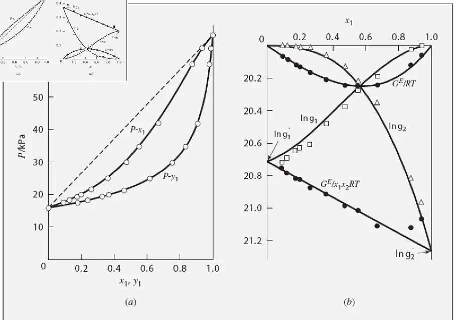
Binary system acetonitrile (1)/nitromethane(2) conforms closely to Raoult’s law. Vapor pressures for the pure species are given by the following Antoine equations:

(a) Prepare a graph showing P vs. x₁ (bubble point-line) and P vs. y₁ (dew

point-line) for a temperature of 75°C.

(b) Prepare a graph showing T vs. x₁ (bubble point-line) and T vs. y₁ (dew

point-line) for a pressure of 70 kPa.

00 . 224 / 47 . 2945 2724 . 14 / ln ₁    C t kPa Psat _ 00 . 209 / 64 . 2972 2043 . 14 / ln ₂    C t kPa Psat _

Example 10.1

)

...,

,

2

,

1

(

i

N

P

x

P

y

_i



_{i i}sat



)

...,

,

2

,

1

(

i

N

P

x

P

i sat i i







1 



i i y Binary system 1 2 1 2

(

P

P

)

x

P

P



sat



sat



sat

1 



i i x ) ..., , 2 , 1 ( / 1 N i P y P i sat i i  



For dewpoint calculation

- Liquid phase composition is unknown

Calculation procedure :

For bubblepoint calculation

- vapor phase composition is unknown

sat i i

x P

y

P



i i sat i

y P

x

P



BULB P DEW P 1 1 2 2

1

/

sat

/

sat

P

y P

y

P





(a) i) BULB P : known properties ; T(= 75°C) and x₁(= 0.6) unknown properties : P and y₁

1 2

1

2

(

P

P

)

x

P

P



sat



sat



sat

21

.

83

1



sat

P

At 75°C

P

₂sat



41

.

98

1

)

98

.

41

21

.

83

(

98

.

41

x

P







e.g. x1 = 0.6 0.7483 72 . 66 ) 21 . 83 )( 6 . 0 ( 1 1 1    P P x y sat 72 . 66  P

Therfore, at 75°C, a liquid mixture of 60 mol-% (1) and 40 mol-% (2) is in equilibrium with a vapor containing 74.83 mol-% (1) at pressure of 66.72 kPa.

Ref. => Fig. 10.11 => next slide

Example 10.1(solution)

by Antoine eqn. 00 . 224 / 47 . 2945 2724 . 14 / ln ₁    C t kPa Psat _ 00 . 209 / 64 . 2972 2043 . 14 / ln ₂    C t kPa Psat _

(A)

(a) ii) DEW P : known properties ; T(= 75°C) and y₁(= 0.6) unknown properties : P and x₁

21 . 83 1  sat P At 75°C 98 . 41 2  sat P e.g. y₁ = 0.6 1 1 1

(0.6)(59.74)

83.21

0.4308

sat

y P

x

P







59.74

P



Therfore, at 75°C, a vapor mixture of 60 mol%(1) and 40 mol%(2) is in equilibrium with a liquid containing 43.08 mol% (1) at pressure of 59.74 kPa. => Liquid-phase composition at point c'

Ref. => Fig. 10.11 => next slide

Example 10.1

by Antoine eqn. 1 2 1 2

1

Sat Sat

P

y

y

P

P





1 59.74 0.6 / 83.21 0.4 / 41.98 P   kPa 

Ideal Phase Behaviour: P - x - y Diagrams

T=75ºC x₁=0.6 _{P=66.72 kPa} y1=0.7483 T=75ºC y₁=0.6 P=59.74 kPa x1=0.4308 Given as Given as DEW P BUBL P

Calculation procedure : T – x – y calculation

sat sat sat

P

P

P

P

x

2 1 2 1







Simple method of plotting T – x – y

ln

sat i i i i

B

t

C

A

P







Select t sat

P

₁ sat

P

₂ t vs. x₁ t vs. y₁

• Given p, xi (or yi) for all components Find T, yi (or xi) for all components

Select t between and

t

₁sat

t

₂sat

1 2 1 2 1

(

)

(

)

sat sat sat sat

P

P

P

y

P P

P







1 2 1 2

(

P

P

)

x

P

P



sat



sat



sat

1 1 2 2

1

/

sat

/

sat

P

y P

y

P





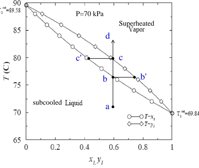
Fig. 10.12 txy diagram of acetonitrile(1)-nitromethane(2) at 70kPa d c b' b c' a subcooled Superheated P=70 kPa

53

BULB T(known; x

_i

, P) by

=>1st _{see next slide}

Iteration procedure

• Calc

• Calc by eqn. B←

• Calc t for 2-comp by Antoine eqn.

• Determine a new by eqn. C

• Calc yi…

1 2 1 2 1 2 1 2 ln lnPsat ln Psat A A B B t C t C          2 sat

P

2

2972.64

209.00

14.2043 ln

sat

t

P







2 1 2 sat

P

P

x



x





1 2 1 2 1 2 1 2 ln lnPsat ln Psat A A B B t C t C         





sat 2 sat 1 T T T  '  i i i sat i C P A B T    ) ln( 1 2 1 ( ) 2 sat sat t  T T

←

←



(0.6)(87.17) 0.7472 70 sat i i i x P y P   

(b) BUBL T, having x₁=0.6, P = 70 kPa

2945.47 2972.64 ln 0.0681 224.00 209.00 t t       t = 76.42ºC = 87.17 kPaP₁sat

(B)

(C)

(C)

Check (t

_n-1

-t

_n

)

1 1 1 1 2 2 2 2 sat sat ij sat sat y x P P P y x P P P



   2 1 2 1 1 1 1 2 2 2 2 2 1 1 2 1 1 1 2 ( ) 1 ( 1) , 1 ( 1) 1 ( 1)

sat sat sat

sat sat

sat sat sat

sat sat P P P P x P P P x P P P P x P P P x P x x x x P x x                         1

(

1 2

)

sat

P



P y



y



1 2 1 2 2 1 1 2 1 2 1 1 2 1 2 _{1 2 1 2} 1 1 1 2

1

1

1

/

_/

(

)

sat sat sat sat sat sat

sat

sat sat _{sat sat} sat sat

P

y

y

y P

y P

P

P

P P

P

y

y P

P

_y

_{y P}

_P

P

P

P y

y

















_







(B)

2 1 2 sat

P

P

x



x





DEW T(known; y

_i

, P) by

1

(

1 2

)

sat

P



P y



y



←



Iteration procedure

• Calc

Calc

• Calc t for 1-comp by Antoine eqn.

• Determine a new

• Calc x

_i 1 2 1 2 1 2 1 2 ln lnPsat ln Psat A A B B t C t C          1 sat

P

1

2945.47

224.00

14.2724 ln

sat

t

P







1 2 1 2 1 2 1 2 ln lnPsat ln Psat A A B B t C t C         





sat 2 sat 1 T T T  '  i i i sat i C P A B T    ) ln( 1 2 1 ( ) 2 sat sat t  T T

←

←

1

(

1 2

)

sat

P



P y



y



(0.6)(70) 0.4351 96.53 i i _sat i y P x P   

(b) DEW T, having y₁=0.6, P = 70 kPa

2945.47 2972.64 ln 0.0681 224.00 209.00 t t       t = 79.58ºC = 96.53 kPaP₁sat

←

Check (t

_n-1

-t

_n

)

VLE in Binary Systems

Alternately, we can specify a system pressure (often atmospheric) and examine VLE behaviour as a function of temperature and

composition.

Acetonitrile(1) Nitromethane(2) @ 70kPa

65.0 70.0 75.0 80.0 85.0 90.0 0.00 0.20 0.40 0.60 0.80 1.00 x1,y1 T e m p , d e g C y1 x1 x₁=0.6, P = 70 kPa y₁=0.7472, T = 76.42ºC

BUBL T

y₁=0.6, P = 70 kPa X₁=0.4351, T = 79.58ºC

DEW T

Gas-Liquid Equilibrium – Henry’s Law

• In the previous discussions, both components could exist

as a pure liquid at the temperatures of interest

• In other words we were interested in vapor-liquid

equilibria

• How can we extend this discussion to include gas-liquid

equilibria,

for species that do not condense

Henry’s law

Raoult’s law를 사용하기 위해서는 의 값이 필요.  적용온도(25ºC)가 임계온도 이하여야 함(∵ 증기압계산이 가능함)  적용온도 >> 공기의 임계온도(-140.95℃) => 증기압을 계산할 수 없음 Ex) 공기(1) 중의 물(2) 증기의 분율(y₂);  Raoult’s law을 물에 적용 하여 구함 » 가정 : 공기가 액상 중에 용해되지 않는다  물(액체물은 순수한 것으로 가정)에 대한 Raoult’s law ; Ex) 물(2)속에 용해된 공기(1)의 분율(x₁);  적용온도 (25ºC) >> 공기의 임계온도 => Raoult’s law을 적용할 수 없음.  ∴ Henry’s law를 이용하여 해결 - 기상을 이상기체로 간주(충분히 낮은 압력에 적용 가능)  액상 중에 아주 희박한 용질로서 존재하는 성분에 대해 적용(예, 물속의 공기 등)  기상 중의 성분의 분압은 그 성분의 액상 몰분율에 직접 비례한다. H x P y  sat i

P

2 2 2 (1)(3.166) 0.0312 101.33 sat x P y P    물의 증기압, at 25ºC

air H₂O x1(액상,air) y2(기상,water) x2(액상,물) y1(기상,공기) 1 1 1 sat y P x P 

Henry’s law

•

Henry’s law :

 기상 중의 성분의 분압은 그 성분의 액상 몰분율에 직접 비례한다. » ; Henry’s constant • 25ºC 대기압 하에서의 공기(1)/물(2) 계에 대해

 y₁=1-y₂=1-0.0312=0.9688인 공기(1)에 Henry’s law를 적용하면, •Check unit !! i H 5 1 1 1

(0.9688)(101.33)

1.35 10

72,950

y P

x

H











i i i

P

x

H

y



From Table 10.1

x1: mole fraction of air in water

■Example 10.2 Assuming that carbonated water contains only CO₂ (species 1) and H₂O (species 2) , determine the compositions of the vapor and liquid phases in a sealed can of “soda” and the pressure exerted on the can at 10°C. Henry’s

constant for CO₂ in water at 10°C is about 990 bar. Henry’s law for species 1: y1P  x1H1

Raoult’s law for species 2: sat

P x P y₂  _{2 2} sat P x H x P  _{1 1}  _{2 2} Assuming x₁ = 0.01

(0.01)(990) (0.99)(0.01227)

9.912 bar

P







1 1 1P x H y  _{assuming y1 ≡ 1.0} 01 . 0 1  x sat P x P y₂  _{2 2} 0012 . 0 2  y 9988 . 0 1 

y Justified the assumption

almost pure CO

Justified the assumption

CO₂ : species 1

H₂O : species 2

From steam table at 10°C

1 1 9.912 0.0100 990 P x H    2 2 2 (0.99)(0.01227) 0.0012 9.912 sat x P y P   

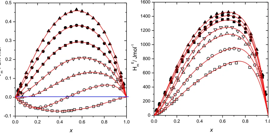
10.5 VLE modified Raoult’s law

Account is taken of deviation from solution ideality in the liquid phase by a factor inserted into Raoult’s law:

) ... , 3 , 2 , 1 (i N P x P y_i  _i



_{i i}sat 

The activity coefficient, f (T, x

_i

)



 i sat i i i P x P





 i sat i i i P y P



/ 1

Example 10.3 For the system methanol (1)/methyl acetate (2), the following

equations provide a reasonable correlation for the activity coefficients:

2 1 2 2 2

ln

(2.771 0.00523 )

Ax

T x









2 2 1 2 1 ln (2.771 0.00523 ) Ax T x



  

The Antoine equations provide vapor pressures:

424 . 33 ) ( 31 . 3643 59158 . 16 / ln ₁    K T kPa Psat 424 . 53 ) ( 54 . 2665 25326 . 14 / ln ₂    K T kPa Psat Calculate

(a): P and {y_i} for T = 318.15 K and x₁ = 0.25 (b): P and {x_i} for T = 318.15 K and y₁ = 0.60 (c): T and {y_i} for P = 101.33 kPa and x₁ = 0.85 (d): T and {x_i} for P = 101.33 kPa and y₁ = 0.40

Solution 10.3

(a) for T = 318.15, and x₁ = 0.25 51 . 44 1  sat P P₂sat 65.64 50 . 73 ) 64 . 65 )( 072 . 1 )( 75 . 0 ( ) 51 . 44 )( 864 . 1 )( 25 . 0 (    



i sat i i i P x P



sat i i i iP x P y 



y₁  0.282 y₂ 0.718 By Antoine eqn. 864 . 1 1   ₂ 1.072 2 2 1 (2.771 0.00523 ) ln   T x 2 1 2 (2.771 0.00523 ) ln   T x

=> no difference with simple Raoult’s law

γ=f(x,T)

BUBL P calc

A iterative process is applied, with ₁ 1 ₂ 1 



i sat i i i P y P



/ 1 sat P P y x 1 1 1 1 



x₂ 1 x ₁

Converges at: P  62.89 kPa ₁ 1.0378 ₂  2.0935 x₁ 0.8169

1 1 1 2 2 2

1

sat sat

P

y



P

y



P





(b): for T = 318.15 K and y₁ = 0.60 Initial values 2 2 1 (2.771 0.00523 ) ln   T x 2 1 2 (2.771 0.00523 ) ln   T x 2nd _step, 51 . 44 1  sat P P₂sat 65.64 By Antoine eqn.

γ=f(x,T)

=> no x

_i Check (P_n-1-P_n) Approx. value

DEW P Calc

424 . 33 ) ( 31 . 3643 59158 . 16 / ln ₁    K T kPa Psat 424 . 53 ) ( 54 . 2665 25326 . 14 / ln ₂    K T kPa Psat

(c): for P = 101.33 kPa and x₁ = 0.85

by

with α

71 . 337 1  sat T T₂sat 330.08

A iterative process is applied, with T (0.85)T₁sat (0.15)T₂sat 336.57

... 1   ₂ ... 1 1 1 2 2 sat

P

P

x



x

 





  1.0236  2.1182 y 0.670 y  0.330 ln( ) sat i i sat i i i B T C A P    101.33 P  kPa 1 2 1 2 1 2 1 2 ln ln sat ln sat B B P P A A t C t C          1 2 ln  Psat Psat 2nd _step sat i i i i x P y P  

γ=f(x,T)

=> no T

Check (Psat n-1-Psatn) New T 2 2 1 (2.771 0.00523 ) ln   T x 2 1 2 (2.771 0.00523 ) ln   T x

BULB T calc

(d): for P = 101.33 kPa and y₁ = 0.40 71 . 337 1  sat T T₂sat 330.08

A iterative process is applied, with T (0.40)T₁sat (0.60)T₂sat 333.13

1 1   ₂ 1 ... 1  sat P



 i sat i i i P x P  i i i sat i C K T B A kPa P    ) ( / ln Converges at: T 326.70K  1.3629  1.2523 x 0.4602 x 0.5398 ... 2  sat P ... 1  x x₂ ... ... 1   ₂ ... ... 1  sat P 1 2 1 1 2 ln sat y y P P       _  _  

Saturation Temps. are the same as part (c)

Initial Values; 1 2 ln  Psat Psat 1 i i sat i y P x P   2 2 1 (2.771 0.00523 ) ln   T x 2 1 2 (2.771 0.00523 ) ln   T x 1 1 1 ln 1 sat B T C A P    γ=f(x,T) => no x,T 1 2 1 1 2 ln sat y y P P       _  _   Check (T_n-1-T_n)

DEW T calc

(e): the azeotropic pressure and the azeotropic composition for T = 318.15 K

Define the relative volatility:

2 2 1 1 12 x y x y   Azeotrope y1  x1 y2  x2 12 1 sat i i i i y P  x



P sat sat P P 2 2 1 1 12     1 1 1 1 1 12 1 ₂ 2 2 2 1 2 0.224 exp( ) exp(2.771 0.00523 )

sat sat sat

x _{sat sat sat}

P P P P P Ax P T        _  2 2 1, 1 exp(Ax2 )     2 1 1, 2 exp(Ax1 )     1 2 1 1 1 2 1 12 0 2 2 2 2 exp( ) exp(2.771 0.00523 ) 2.052

sat sat sat

x _{sat sat sat}

P P Ax P T P P P         

Since α₁₂ is a continuous function of x₁: from 2.052 to 0.224, α₁₂ = 1 at some point There exists the azeotrope!

1 1 1 12  sat  sat P P    1 2 65.64 1.4747 az sat az sat P      2 1 2

ln





Ax

2 ln



 Ax

From Antoine eq.

1 2 , 0 1 when x   x  when x, ₂  0 x₁1 2 2 exp(Ax1 )   2 1 exp(Ax2)   1 1 1 1 sat y x  P P

1 2 2 1 1 12  sat  sat P P    1 2 2 1 65.64 1.4747 44.51 az sat az sat P P      2 2 1

(

2

.

771

0

.

00523

)

ln







T

x

2 1 2

(

2

.

771

0

.

00523

)

ln







T

x

2 2 1 2 1 2 1 2 1 2 2 1 1 1 1 ln ( )( ) ( ) (2.771 0.00523 )(1 2 ) ln1.4747 0.388 1.107(1 2 ) 0.388 0.325 Ax Ax A x x x x A x x T x x x





                az az

y

x

₁



0

.

325



₁ 1

exp(

22

)

exp(1.107 (1 0.325) )

2

1.657

az

Ax







 



1 1 (1.657)(44.51) 73.76 az az sat P  P   kPa 2 1 2

ln





Ax

2 2 1 ln



 Ax sat i i i i y P  x



P

10.6 VLE from K-value correlations

A convenient measure, the K-value:

 the “lightness” of a constituent species, i.e., of its tendency to favor the vapor phase.

 When K_i > 1, species i => higher concentration in vapor phase

 When K_i < 1, species i => higher concentration in liquid phase,

and is considered a “heavy” constituent  The Raoult’s law and modified Raoult’s law :

 For bubble point calc,

for dew point calc i i i x y K  , 1 sat i i i i sat i i i i i i i i i i i i i y P x P y P K y K x x P y y x x K K             sat i i i sat i i i i

y P x P

y

P

K

x

P



 

1 i i y K  

1

i i i

K x





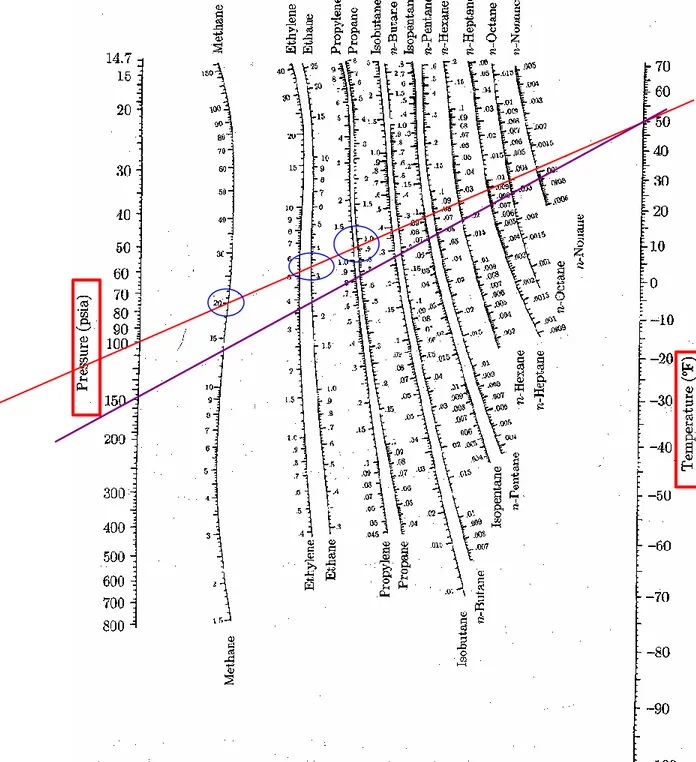
Fig. 10.13 K-values for

systems of light hydocarbons.

Example 10.4 For a mixture of 10 % methane, 20 % ethane, and 70

mol-% propane at 50°F, determine: (a) the dewpoint pressure, (b) the bubblepoint

pressure. The K-values are given by Fig. 10.13.

(a) at its dewpoint, only an insignificant amount of liquid is present:

P = 100 (psia) P = 150 (psia) P = 126 (psia)

Species yi Ki yi /Ki Ki yi /Ki Ki yi /Ki

Methane 0.10 20.0 0.005 13.2 0.008 16.0 0.006 Ethane 0.20 3.25 0.062 2.25 0.089 2.65 0.075 Propane 0.70 0.92 0.761 0.65 1.077 0.762 0.919 Σ(yi /Ki) = 0.828 Σ(yi /Ki) = 1.174 Σ(yi /Ki) = 1.000

(b) at bubblepoint, the system is almost completely condensed:

P = 380 (psia) P = 400 (psia) P = 385 (psia)

Species xi Ki xi Ki Ki xi Ki Ki xi Ki Methane 0.10 5.60 0.560 5.25 0.525 5.49 0.549 Ethane 0.20 1.11 0.222 1.07 0.214 1.10 0.220 Propane 0.70 0.335 0.235 0.32 0.224 0.33 0.231 Σ(xi Ki) = 1.017 Σ(xi Ki) = 0.963 Σ(xi Ki) = 1.000 액상의 경우, dew point 보다 낮은 압력에서는 Sx_i<1, 높은 압력에서는 Sx_i>1

1

i i i

K x





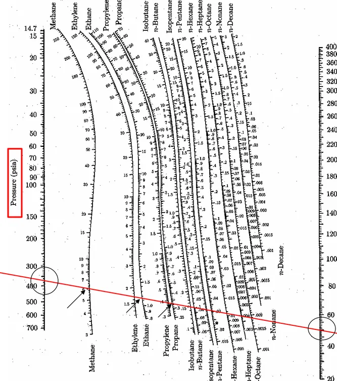
1 i i i y K  

Fig. 10.14 K-values for

systems of light hydocarbons.

Example 10.4

Calculation by Excel

a) dewpoint pressure

species yi Ki yi/Ki Ki yi/Ki Ki yi/Ki

Methane 0.1 20 0.005 13.2 0.008 16 0.006

Ethane 0.2 3.25 0.062 2.25 0.089 2.65 0.075

Propane 0.7 0.92 0.761 0.65 1.077 0.762 0.919

∑(yi/Ki)= 0.827 1.173 1.000

b) bubblepoint pressure

species xi Ki Ki*xi Ki Ki*xi Ki Ki*xi

Methane 0.1 5.6 0.560 5.25 0.525 5.49 0.549

Ethane 0.2 1.11 0.222 1.07 0.214 1.1 0.220

Propane 0.7 0.335 0.235 0.32 0.224 0.33 0.231

∑(Ki*xi)= 1.017 0.963 1.000

P=100(psia) P=150(psia) P=126(psia)

T, P Flash Calculation

 A liquid at a pressure equal to or greater than its bubble point pressure “flashes” or partially evaporates when the pressure is reduced,

producing a two-phase system of vapor and liquid in equilibrium.

 Consider a system containing one mole of non reacting chemical species:  The general nature of a flash calculation is :

 Temperature-Pressure Flash: (T, P, z) => (V, x, y)

zi

F

y

i

V

x

i

L

0 _{x, y} 1 VAPOR LIQUID  P P B P _A A B T = const. x y b r bubble   _dew

Flash Calculations

Liquid Vapour

F

V

L

T, P

F can be a liquid, a gas or a two phase mixture This is called a flash calculation, because if the pressure is reduced enough, the liquid changes to vapor in a “flash”

Flash Calculations

Given a temperature and pressure and an overall composition, => we can calculate x_i and y_i

Consider a system containing 1 mole of liquid:

• z_i = the overall composition

• L =moles of liquid, with mole fractions x_i • V =moles of vapor, with mole fractions y_i

•

The material balance equations are:

. Note: The solution V = 1 is always a trivial solution.

1 ( 1, 2, , ) i i i L V z x L y V i N      (1 ) ( 1, 2, , ) (1 ) 1 (1 ) 1 _{(1 ) (1 ) 1 ( 1)} (1 ) i i i i i i i i i i i i i i i i i i i i i i z x V y V i N y z V y V K z y V V K z z K z K z K y V K V V K V V K V V K           _   _               ( 1, 2, , ) 1 ( 1) i i i i z K y i N V K     L을 제거

and solving for

i i i i x  y K y 1 1 ( 1) i i i i z K V K     1 



i i y Liquid Vapour

F

V

L

T,

P

, sat sat i i i i i i i y P y P x P K x P    Ref.

Flash calculations(Summary)

The moles of liquid

1





V

L

_z

_i



_x

_i

_L



_y

_i

_V

The moles of vapor

The liquid mole fraction

The vapor mole fraction

V

y

V

x

z

_i



_i

(

1



)



_i ) 1 ( 1   i i i i K V K z y 1 ) 1 ( 1  



i i i K V K z

zi

F

y

i

V

x

i

L

0 x, y 1 VAPOR LIQUID  P P B P _A A B T = const. x y b r bubble   _dew

Example 10.5 The system acetone (1)/acetonitrile (2)/nitromethane(3) at 80°C and 110 kPa has the overall composition, z₁ = 0.45, z₂ = 0.35, z₃ = 0.20, Assuming that Raoult’s law is appropriate to this system, determine L, V, {x_i}, and {y_i}. The vapor pressures of the pure species are given.

First, do a BUBL P calculation, with {z_i} = {x_i} :

kPa P x P x P x

P_bubl  _{1 1}sat  _{2 2}sat  _{3 3}sat (0.45)(195.75)(0.35)(97.84)(0.20)(50.32) 132.40

Second, do a DEW P calculation, with {z_i} = {y_i} :

kPa P y P y P y

P_{dew sat sat sat} 101.52

/ / / 1 3 3 2 2 1 1    

Since P_dew < P = 110 kPa < P_bubl, the system is in the two-phase region, sat i i i i y P K x P   1 1.7795 195.75 110 K   8895 . 0 2  K K₃  0.4575 1 ) 1 ( 1  



i i i K V K z mol V  0.7364 ) 1 ( 1   i i i i K V K z y 5087 . 0 1  y 3389 . 0 2  y 1524 . 0  y mol V L 1  0.2636 i i i i i y K x y x K    2859 . 0 1  x 3810 . 0 2  x 3331 . 0  x

1

st

2

nd

3

rd

Example 10.5

Calculation by Excel A B C Vapor Pressure Acetone 14.3145 2756.22 228.06 214.32 195.75 Acetonitrile 14.895 3413.1 250.523 96.41 97.84 Nitromethane 14.7513 3331.7 227.6 50.40 50.32 Temp/℃ 80 P/kPa 110 calc V 0.8107 0.7365

overall composition Eqn. 10.17 -7.6126E-08 -5.49479E-08

z1 0.45 z2 0.35 L 0.1893 0.2635 z3 0.2 y1 0.4957 0.5087 Pbubl/kPa 140.2694 132.40 1) y2 0.3409 0.3389 Pdew/kPa 103.1141 101.52 2) y3 0.1634 0.1524 K1 1.9484 1.7795 x1 0.2544 0.2859 K2 0.8765 0.8895 x2 0.3889 0.3810 K3 0.4582 0.4575 x3 0.3566 0.3331

Antoine Constants Given Values in Textbook

3)

4)

5)

Example 10.6

반복법에 의한 해

P/kPa 200 yi for _ν= yi for _ν= yi for _ν= yi for _ν=

해찾기에 의한 결 과 xi=yi/Ki for v=0.273 zi Ki 0.3500 0.2500 0.2700 0.2730 0.2500 Methane 0.1 10 0.2410 0.3077 0.2915 0.2893 0.3077 0.0308 Ethane 0.2 1.76 0.2780 0.2958 0.2921 0.2915 0.2958 0.1681 Propane 0.7 0.52 0.4375 0.4136 0.4182 0.4189 0.4136 0.7955 Σyi 0.9565 1.0171 1.0018 0.9997 1.0171 0.9943 Σxi

Calculation by Excel

Example

Assuming Roult’s Law to be valid, prepare (a)a Pxy diagram for T=90o_{C, and}

(b)a Txy diagram for P=90 kPa

for a mixture of 1-chlorobutane (1) /chlorobenzene (2) Antoine Coefficients:

A B C

1-chlorobutane (1) 13.9600 2826.26 224.10