Chapter 15. Dynamic Behavior of Thermal Systems

(1)

Min Soo KIM

Department of Mechanical and Aerospace Engineering Seoul National University

Optimal Design of Energy Systems ( M2794.003400 )

Chapter 15. Dynamic Behavior of

Thermal Systems

(2)

Chapter 15. Dynamic Behavior of Thermal Systems

15.1 In What Situations is Dynamic Analysis Important?

Steady-state Dynamic

More frequently than dynamic simulations Can be justified in the design

Ex. Part-load efficiency,

Potential operating problems

Address transient problems Can be corrected in in the field

Ex. System shutdown, Damage the plant, Imprecise control

Dynamic Analysis : with respect to time, on/off, under control, disturbance

(3)

Chapter 15. Dynamic Behavior of Thermal Systems

15.2 Scope and Approach of This Chapter

Intention

Concentration on thermal components Emphasis of behavior in the time domain

The translation of physical situations into symbolic or mathematical representation

Object

More comfortable in making dynamic analysis

Representation of the performance in the time domain Experience in block diagram

(4)

Chapter 15. Dynamic Behavior of Thermal Systems

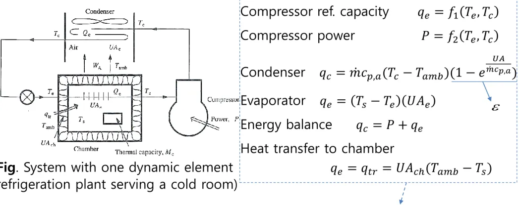
15.3 One Dynamic Element in a Steady-State Simulation



steady-state

Fig. System with one dynamic element (refrigeration plant serving a cold room)

Compressor ref. capacity 𝑞_𝑒 = 𝑓₁ 𝑇_𝑒, 𝑇_𝑐 Compressor power 𝑃 = 𝑓₂ 𝑇_𝑒, 𝑇_𝑐 Condenser 𝑞_𝑐 = 𝑚𝑐_𝑝,𝑎(𝑇_𝑐 − 𝑇_𝑎𝑚𝑏)(1 − 𝑒

𝑈𝐴 𝑚𝑐𝑝,𝑎) Evaporator 𝑞_𝑒 = 𝑇_𝑠 − 𝑇_𝑒 𝑈𝐴_𝑒

Energy balance 𝑞_𝑐 = 𝑃 + 𝑞_𝑒 Heat transfer to chamber

𝑞_𝑒 = 𝑞_𝑡𝑟 = 𝑈𝐴_𝑐ℎ(𝑇_𝑎𝑚𝑏 − 𝑇_𝑠)

(5)

15.3 One Dynamic Element in a Steady-State Simulation

Pull-down 𝑞_𝑡𝑟 = 𝑈𝐴_𝑐ℎ 𝑇_𝑎𝑚𝑏, −𝑇_𝑠 𝑞_𝑡𝑟 = 𝑞_𝑒 + 𝑚𝑐_𝑝 ^𝑑𝑇^𝑠

𝑑𝑡

Dynamic : during pull-down 𝑞_𝑡𝑟 ≠ 𝑞_𝑒 𝑇_𝑠

𝑞_𝑡𝑟 𝑞_𝑒

𝑚, 𝑐_𝑝

(6)

15.4 Laplace transform

Powerful tool in predicting dynamic behavior One way to solve ODE

𝐿 𝐹 𝑡 =

0

∞

𝐹 𝑡 𝑒^−𝑠𝑡𝑑𝑡 = 𝑓(𝑠)

𝐿 𝐹′ 𝑡 =

0

∞

𝐹′ 𝑡 𝑒^−𝑠𝑡𝑑𝑡

= 𝑒^−𝑠𝑡𝐹(𝑡)]₀^∞- ₀^∞𝐹(𝑡)(−𝑠) 𝑒^−𝑠𝑡𝑑𝑡

= −𝐹 0 + 𝑠𝑓(𝑠)

𝐿 𝐹′′ 𝑡 =

0

∞

𝐹′′ 𝑡 𝑒^−𝑠𝑡𝑑𝑡

= 𝑒^−𝑠𝑡𝐹′(𝑡)]₀^∞- ₀^∞𝐹′(𝑡)(−𝑠) 𝑒^−𝑠𝑡𝑑𝑡

= −𝐹′ 0 + 𝑠[−𝐹 0 + 𝑠𝑓 𝑠 ]

= −𝐹^′(0) − 𝑠𝐹(0) + 𝑠²𝑓 𝑠

(7)

15.4 Laplace Transforms

Example 15.1 : What is the Laplace transform of the constant c ? (Solution)

𝓛{c} = ₀^∞𝑐 𝑒^−𝑠𝑡𝑑𝑡 = −^𝑐

𝑠 𝑒^−𝑠𝑡]₀^∞=^𝑐

𝑠

Example 15.2 : What is the Laplace transform of bt ? (Solution)

𝓛{bt} = ₀^∞𝑏𝑡 𝑒^−𝑠𝑡𝑑𝑡 = −𝑏 ^𝑑

𝑑𝑠 0

∞𝑒^−𝑠𝑡𝑑𝑡 = −𝑏^𝑑(¹ ^𝑠⁾

𝑑𝑠 = 𝑏/𝑠²

(8)

15.5 Inversion of Laplace Transforms 𝐿

⁻¹

𝑓 𝑠 = 𝐹(𝑡)

Example 15.4 : Invert 𝑠+10 (𝑠−2)²(𝑠+1)

(Solution) 𝑠+10

(𝑠−2)²(𝑠+1)

=

^𝐴

(𝑠+1)

+

^𝐵

(𝑠−2)²

+

^𝐵′

𝑠−2 𝑐𝑜𝑛𝑠𝑡𝑎𝑛𝑡𝑠 ∶ 10 = 4𝐴 + 𝐵 − 2𝐵^′

𝑠 ∶ 1 = −4𝐴 + 𝐵 − 𝐵^′ 𝑠² ∶ 0 = 𝐴 + 𝐵^′ 𝐴 = 1, 𝐵 = 4, 𝐵^′ = −1

∴ 𝐿

⁻¹ ^𝑠+10

(𝑠−2)²(𝑠+1)

= 𝑒

^−𝑡

+ 4𝑡𝑒

^2𝑡

− 𝑒

^2𝑡

(9)

15.5 Inversion of Laplace Transforms 𝐿

⁻¹

𝑓 𝑠 = 𝐹(𝑡)

(Another Solution of Example 15.4)

 For non-repeated roots 𝑁(𝑠)

𝐷(𝑠)

=

^𝐴

𝑠−𝑎

+

^𝐵

𝑠−𝑏

+ ⋯ 𝐴 =

^{𝑁(𝑠)(𝑠−𝑎)}

𝐷(𝑠)

│

_𝑠→𝑎

𝐵 =

^{𝑁(𝑠)(𝑠−𝑏)}

𝐷(𝑠)

│

_𝑠→𝑏

 For repeated roots 𝑁(𝑠)

𝐷(𝑠)

=

^𝐴

𝑠−𝑎

+

^𝐵

(𝑠−𝑏)²

+

^𝐵′

𝑠−𝑏

𝐵 =

^{𝑁(𝑠)(𝑠−𝑏)}²

𝐷(𝑠)

│

_𝑠→𝑏

𝐵′ =

^𝑑

𝑑𝑠

[

^{𝑁(𝑠)(𝑠−𝑏)}²

𝐷(𝑠)

]

_𝑠→𝑏

→ 𝐴 =

^𝑠+10

(𝑠−2)²

│

_𝑠→−1

= 1 𝐵 =

^𝑠+10

𝑠+1

│

_𝑠→2

= 4 𝐵

^′

=

^𝑠+10

𝑠+1

│

_𝑠→2

= −1

(10)

15.6 Solution of ordinary differential equations

Example 15.6 : Solve 𝒀^′′ 𝒕 + 𝒌^𝟐𝒀 𝒕 = 𝟎

(boundary conditions : Y(0) = A, Y’(0) = B) (Solution)

Transform the differential equation 𝑠²𝑦 𝑠 − 𝑠𝑌 0 − 𝑌^′ 0 + 𝑘²𝑦 𝑠 = 0 Boundary conditions

𝑦 𝑠 = 𝐴𝑠

𝑠² + 𝑘² + 𝐵 𝑠² + 𝑘² Invert y(s)

𝑌 𝑡 = 𝐴𝑐𝑜𝑠 𝑘𝑡 + (𝐵/𝑘)𝑠𝑖𝑛(𝑘𝑡)

(11)

15.7 Blocks, Block diagrams, and transfer functions

Transfer function : 𝑇𝐹 = 𝐿{𝑂 𝑡 }

𝐿{𝐼 𝑡 } = 𝑂(𝑠)

𝐼(𝑠)

ratio of the output to the input

- Variable in S domain (not in time domain)

Fig. Symbols used in block diagrams Fig. Transfer function and cascading of blocks

Proper T.F. = 분모 차수 ≥ 분자 차수

(12)

15.7 Blocks, Block diagrams, and transfer functions

Transfer function : 𝑇𝐹 = 𝐿{𝑂 𝑡 }

𝐿{𝐼 𝑡 } = 𝑂(𝑠)

𝐼(𝑠)

ratio of the output to the input

- Variable in S domain (not in time domain)

mu(t) x(t)

𝑢 𝑡 + 𝑚𝑔 − 𝑘 ∗ 𝑥 𝑡 = 𝑚𝑥(𝑡)

0 − 𝑘𝛿𝑥 + 𝛿𝑢 = 𝑚 𝛿𝑥

Inverse Laplace −𝑘∆𝑋 𝑠 + ∆𝑈 𝑠 = 𝑚𝑠²∆𝑋(𝑠)

𝑇𝐹 = ∆𝑋(𝑠)

∆𝑈(𝑠) = 1 𝑚𝑠² + 𝑘

(13)

15.8 Feedback Control Loop

Unity feedback

𝑇𝐹 =

^𝐺(𝑠)

1+𝐺(𝑠)

Non-unity feedback

𝑇𝐹 =

^𝐺(𝑠)

1+𝐺 𝑠 𝐻(𝑠)

Fig. (a) Unity feedback loop

(b) Nonunity feedback loop

(14)

15.9 Time Constant Blocks

Standard technique for developing transfer function 1. Write differential equation 𝑚𝑐^𝑑𝑇

𝑑𝑡 = 𝑇_𝑓 − 𝑇 ℎ𝐴 2. Transform equation ^𝑚𝑐

ℎ𝐴 𝑠𝐿 𝑇 − 𝑇 0 = 𝐿(𝑇_𝑓) − 𝐿(𝑇) 3. Solve for transfer function (𝐿 𝑂 /𝐿{𝐼}) 𝑇𝐹 = ^𝑇(𝑠)

𝑇_𝑓(𝑠) =

1+𝑇(0) ^𝐵

𝑇𝑓(𝑠)

1+𝐵𝑠 (𝐵 = ^𝑚𝑐

ℎ𝐴) For special case 𝑇 0 = 0 ∶ 𝑇𝐹 = ¹

Fig. (a) Response of a temperature-sensing bulb to a change in fluid temperature (b) Transfer function of this time-constant block

(15)

15.9 Time Constant Blocks

𝑚𝑐 𝑑(𝑇 − 𝑇₀)

𝑑𝑡 = 𝑇_𝑓 − 𝑇₀ − 𝑇 − 𝑇₀ ℎ𝐴 𝑇𝐹 = 𝐿{𝑇 − 𝑇₀}

𝐿{𝑇_𝑓 − 𝑇₀} = 1 𝐵𝑠 + 1

𝑇_𝑓 ∶ unit step increase 𝑇_𝑓 𝑠 = ∆ 𝑠 𝐿 𝑇 − 𝑇₀ = 𝐿 𝑇_𝑓 − 𝑇₀ 1

𝐵𝑠 + 1 = ∆

𝑠(𝐵𝑠 + 1) = ∆ 𝛼

𝑠 − 𝛽

𝐵𝑠 + 1 = ∆(1

𝑠 − 𝐵 𝐵𝑠 + 1)

𝑇 − 𝑇₀ = ∆ 1 − 𝑒⁻^𝐵^𝑡 𝐵 = 𝑚𝑐

ℎ𝐴 ∶ time constant

𝛼𝛽 − 𝛽 = 0, 𝛼 = 1, 𝛽 = 𝐵

(16)

desired temperature

cf) Time Constant Blocks - additional

• Control

• Feedback

• Block diagrams Reference

sensor Actuator process

output sensor

2

-

+ ^control^input ^output

disturbance

desired room

temperature T → V Inverter Refrigeration

system Thermometer

2

-

+ Actual Temp.

Ex)

Chapter 15. Dynamic Behavior of Thermal Systems

(17)

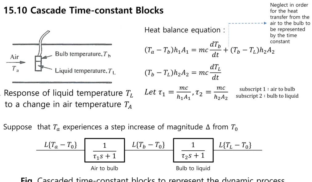
15.10 Cascade Time-constant Blocks

Fig. Response of liquid temperature 𝑇_𝐿 to a change in air temperature 𝑇_𝐴

Heat balance equation :

𝑇_𝑎 − 𝑇_𝑏 ℎ₁𝐴₁ = 𝑚𝑐𝑑𝑇_𝑏

𝑑𝑡 + (𝑇_𝑏 − 𝑇_𝐿)ℎ₂𝐴₂ (𝑇_𝑏 − 𝑇_𝐿)ℎ₂𝐴₂ = 𝑚𝑐𝑑𝑇_𝐿

𝑑𝑡

𝐿𝑒𝑡 𝜏₁ = ^𝑚𝑐

ℎ₁𝐴₁, 𝜏₂ = ^𝑚𝑐

ℎ₂𝐴₂

subscript 1 ∶ air to bulb subscript 2 ∶ bulb to liquid

Neglect in order for the heat transfer from the air to the bulb to be represented by the time constant

Air to bulb Bulb to liquid

𝐿{𝑇_𝑎 − 𝑇₀} 𝐿{𝑇_𝑏 − 𝑇₀} 1 𝐿{𝑇_𝐿 − 𝑇₀} 𝜏₂𝑠 + 1

1 𝜏₁𝑠 + 1

Suppose that 𝑇_𝑎 experiences a step increase of magnitude ∆ from 𝑇₀

(18)

For unit step input

𝐿 𝑇_𝐿 − 𝑇₀ = ∆

𝑠 ( 1

𝜏₁𝑠 + 1)( 1 𝜏₂𝑠 + 1) Inversion

𝑇_𝐿 − 𝑇₀

∆ = 1 − 𝜏₁

𝜏₁ + 𝜏₂𝑒⁻

𝑡

𝜏₁ − 𝜏₂

𝜏₂ + 𝜏₁𝑒⁻

𝑡 𝜏₂

Chapter 15. Dynamic Behavior of Thermal Systems

15.10 Cascade Time-constant Blocks

①𝑡 = 0, 𝑇_𝐿 − 𝑇₀ = 0

② 𝑑(𝑇_𝐿 − 𝑇₀)

𝑑𝑡 = 0 𝑎𝑡 𝑡 = 0

③𝑖𝑓 𝜏₂ ≪ 𝜏₁ 𝑇_𝐿 − 𝑇₀ = ∆(1 − 𝑒^−𝑡/𝜏)

④𝑖𝑓 𝜏₂ = 𝜏₁ ^𝑇^𝐿^−𝑇⁰

∆ = 1 − 𝑒^−𝑡/𝜏 −^𝑡𝑒^−𝑡/𝜏

𝜏

(19)

15.11 Stability Analysis

- Bode diagram expresses the frequency response of the system

- Bode diagram offers an excellent technique for explaining the mechanics of instability

(20)

- The sum of the phase lags around the loop and the product of the amplification ratio are computed

- The principle that leads to the Bode Criterion for stability is based on transmission of sine waves throughout the loop

- Example : Air heater – controlled by a loop that senses the outlet air temperature 𝑇_𝑎 and converts this sensed temperature 𝑇_𝑏 to a control voltage 𝑉_𝑐

(21)

15.11 Stability Analysis

- Air temperature 𝑇_𝑎 experiences a disturbance that is the top half of a sine wave - The sensed temperature 𝑇_𝑏 lags the variation in 𝑇_𝑎 by an angle 𝜙₁

- The variation in 𝑇_𝑏 translates to a half sine wave of 𝑉_𝑠𝑒𝑡 − 𝑉_𝑐, but reversed in sign

(22)

At the frequency f where sum of phase lags = 180^o Fig.(a)

At the frequency f where product of amplitude ratio > 1 Fig.(b)

Phase lag =180^o Amplitude ratio > 1

Chapter 15. Dynamic Behavior of Thermal Systems

the loop becomes unstable

(23)

cf) Bode plot

At Linear time-invariant(LTI) system with transfer function H(s), Bode plot consists of magnitude plot & phase plot

Function of filter

Represent the gain and

phase of a system as a

function of frequency

(24)

ex) TF(s) = s+a

i) s = jw << a ii) s = jw >> a

Magnitude Phase

(degree)

0 a 90

w w

(25)

ex) Why Bode plot?

Magnitude (dB)

Phase (degree) 40

𝑑𝐵 = 20𝑙𝑜𝑔₁₀ 𝑇𝐹(𝑠 = 𝑗𝑤)

Crossover frequency 𝑤_𝑐 ∶ 𝑓𝑟𝑒𝑞𝑢𝑒𝑛𝑐𝑦 𝑤 𝑎𝑡 0𝑑𝐵

w w

0

𝒘_𝒄 𝒘_𝒄

-180

Phase margin

𝒘_𝟏 𝒘_𝟏

Gain margin

(26)

cf) Pole-zero plot

Pole-zero plot shows the location in the complex plane of the poles and zeros of the transfer function of a dynamic system, such as a controller, sensor, filter.

Chapter 15. Dynamic Behavior of Thermal Systems

26

 stability

 causal / anti-causal system

 region of convergence

Representing

(27)

cf) Pole-zero plot

𝑇𝐹 𝑠 = 𝑂(𝑠) 𝐼(𝑠)

Pole : value of s that makes TF(s) -> ∞ zero : value of s that makes TF(s) -> 0 Stable : f(t) -> 0 as t -> ∞

Unstable : f(t) -> ∞ as t -> ∞

Marginally stable : f(t) -> a or oscillation as t -> ∞

ex) TF(s) =

^𝟏

𝒔+𝒂

(𝒑𝒐𝒍𝒆 ∶ 𝒔 = −𝒂)

𝑓 𝑡 = 𝑒^−𝑎𝑡

a>0 : stable

a=0 : marginally stable a<0 : unstable

Inverse Laplace

stable unstable m-stable

(28)

Chapter 15. Dynamic Behavior of Thermal Systems

ex) TF(s) =

^𝒔+𝟏

𝒔^𝟐+𝟐𝒔+𝟐

(𝒑𝒐𝒍𝒆 ∶ 𝒔 = −𝟏 ± 𝒋)

𝑓 𝑡 = 𝑒^−𝑡cos(𝑡)

Inverse Laplace

stable

At proper TF, real negative pole only -> stable

(29)

15.14 Restructuring the Block Diagram

- Reconstructing the block to simplify the loop

1. Combine two transfer function in series

2. Exchange two adjacent summing points

(30)

15.14 Restructuring the Block Diagram

3. Move a summing point upstream or downstream of a block

4. Move a take off point

(31)

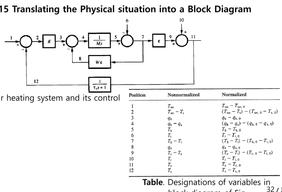
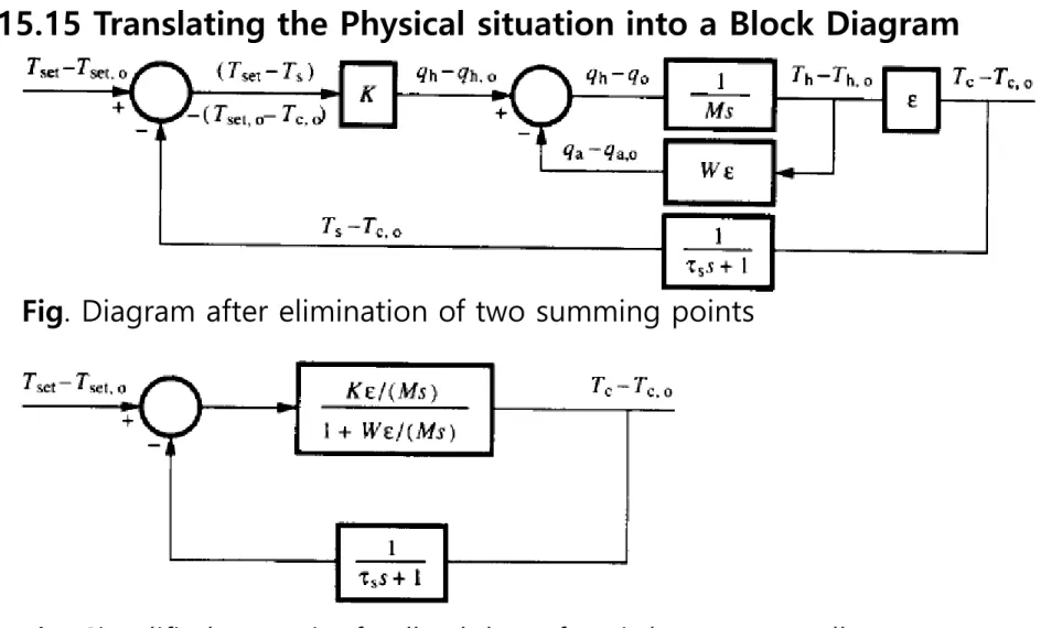
15.15 Translating the Physical situation into a Block Diagram

qa

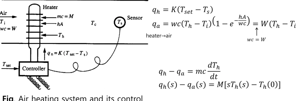
Fig. Air heating system and its control

𝑞_ℎ = 𝐾 𝑇_𝑠𝑒𝑡 − 𝑇_𝑠

𝑞_𝑎 = 𝑤𝑐 𝑇_ℎ − 𝑇_𝑖 1 − 𝑒⁻^ℎ𝐴^𝑤𝑐 = 𝑊(𝑇_ℎ − 𝑇_𝑖)𝜀

heater→air

𝑤𝑐 = 𝑊

𝑞_ℎ − 𝑞_𝑎 = 𝑚𝑐𝑑𝑇_ℎ

𝑞_ℎ(𝑠) − 𝑞_𝑎(𝑠) = 𝑀[𝑠𝑇𝑑𝑡 _ℎ 𝑠 − 𝑇_ℎ 0 ]

(32)

Chapter 15. Dynamic Behavior of Thermal Systems

Fig. Air heating system and its control

Table. Designations of variables in block diagram of Fig. ³² ^{/ 33}

(33)

Fig. Diagram after elimination of two summing points

(34)

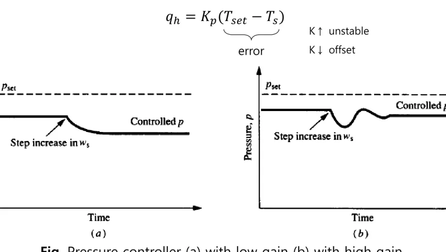
15.16 Proportional Control

error

K↑ unstable K↓ offset

Fig. Pressure controller (a) with low gain (b) with high gain

𝑞

_ℎ

= 𝐾

_𝑝

(𝑇

_𝑠𝑒𝑡

− 𝑇

_𝑠

)

(35)

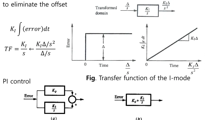
15.17 Proportional – Integral (PI) Control

- to eliminate the offset

- PI control

s



2

KI

s



Fig. Transfer function of the I-mode 𝐾_𝐼 𝑒𝑟𝑟𝑜𝑟 𝑑𝑡

𝑇𝐹 = 𝐾_𝐼

𝑠 ← 𝐾_𝐼∆/𝑠²

∆/𝑠

(36)

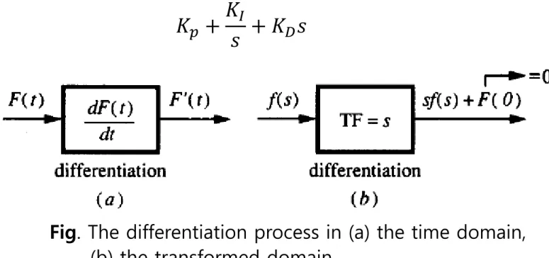
15.18 Proportional-Integral-Derivative(PID) Control

Fig. The differentiation process in (a) the time domain, (b) the transformed domain

𝐾

_𝑝

+ 𝐾

_𝐼

𝑠 + 𝐾

_𝐷

𝑠

(37)

Reaction curve

TF may be approximated by

Time delay of t_d seconds

cf) PID control – Ziegler-Nichols Tuning of PID controller (1942)

𝑒^−𝑡/𝜏

𝐷 𝑠 = 𝐾 1 + 1

𝑇₁𝑠 + 𝑇_𝐷𝑠

𝐾 𝐾

𝑅 =^𝐾

𝜏 : reaction rate

𝐿 = 𝑡_𝑑 𝜏

𝐾 𝜏

𝑇𝐹 = 𝐾𝑒^−𝑡^𝑑 ^𝑆 𝜏𝑠 + 1

(38)

open loop control

cf) Feedforward control

(a) No control

(b) Feed forward control (c) Feedback control