A VAR Model of Stimulating Economic Growth in the Guangdong Province, P.R. China

Abstract

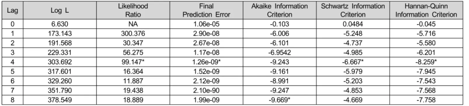
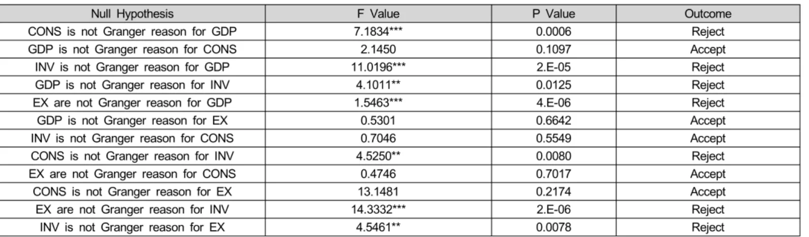
The authors calculate the long-term predictability of GDP, do- mestic demand, investment, and net exports for Guangdong province, P.R. China from 2000 to 2013. A vector autore- gressive (VAR) model with quarterly data for this period is first co-integrated then the Granger causality test is applied to em- pirically assess the relationships among gross domestic product (GDP), consumption, investment, and net exports. There is a strong causality effect between investment and net exports in Guangdong province. However, the variance decomposition re- sults indicate that exports respond to foreign shocks rather than domestic ones, making their impact on the Guangdong economy to predict. Results show the stimulating effect of domestic de- mand on GDP is larger than the stimulating effect of net ex- ports and much larger than even the stimulating effect of investment. The analysis suggests that there are dynamic influ- ences with various levels of persistence between GDP, con- sumption, investment, and net exports. Macroeconomic policy adjustments are urgently required to expand domestic demand and thereby stimulate economic growth in Guangdong province.

Keywords: Economic Growth, Consumption, Investment, Net Exports, VAR Model.

JEL Classification Codes: O40, O53, R11, C51.

* The authors gratefully acknowledge the insightful comments and valuable suggestions made by colleagues from Jinan University in Guangzhou and the Central University of Finance and Economics in Beijing, P.R. China.

** First Author and Corresponding Author, Vice Provost, Global Strategies and Studies, University of Houston [Suite 101, E.W. Cullen Bldg., University of Houston, Houston, TX 77204 USA E-mail: jortiz22

@uh.edu]

*** Visiting Scholar within Global Strategies and Studies, University of Houston, Houston, TX 77204 USA.

**** Professor with the A. R. Sánchez Jr. School of Business, Texas A&M International University, Laredo, TX 78041 USA.

1. Introduction

Active participation in the world economy is often regarded as imperative if countries are to achieve economic growth (Arora 2010; Chang, Kaltani, & Loayza, 2009). International trade raises per-capita income and enhances domestic and foreign competition. Berg, Ostry, and Zettelmeyer (2012) argue that countries that implement export-led strategies also stimulate their imports of technology-intensive manufacturing. Rivera-Batiz and Romer (1991) show that trading goods and ideas allows coun- tries to grow faster due to increasing returns to scale in the re- search and development sector and widened regional market segments. In addition, Hsieh and Klenow (2009) point out that economic growth in East Asia is explained by increases in total factor productivity.

The view that international trade promotes economic growth has been questioned on several grounds. Cline (1982) considers that pursuing export-led strategies is neither a sufficient nor a necessary condition for triggering economic growth, but simply serves as a conduit to it. His critique is based on the dis- advantages that developing countries face in terms of delayed technical know-how and an intricate division of labor. David (1996) suggests that even though exports and investment are both positively correlated among themselves they are, in- dividually speaking, negatively correlated with economic growth for a vast majority of countries.

In the case of East Asian countries, Zhang (2001) argues that it would be a gross over generalization to single out ex- ternal demand as the main factor explaining economic growth.

In fact, almost all developing countries that initially adopted ex- port-led growth strategies found themselves structurally unable to reach high-value-added markets. More worrisome, Paley (2006) maintains East Asian countries that initially pursued export-led growth strategies later experienced negative economic growth.

Dutt and Ghosh (1996) studied the causal relationship be- tween exports and economic growth in five Southeast Asian countries. They found that although economic growth increases exports, the reverse does not hold true. Similarly, Ortiz (2012) measured the sources of economic growth for Latin America in relation to P.R. China. He concluded that Latin American eco- nomic growth was indeed related to the diversification of its ex- port structure. However, growth declined once product diversifi- Print ISSN: 2288-4637 / Online ISSN 2288-4645

doi: 10.13106/jafeb.2015.vol2.no2.5.

A VAR Model of Stimulating Economic Growth in the Guangdong Province, P.R. China*

1)

Jaime Ortiz**, Jingwen Xia***, Haibo Wang****

[Received: March 18, 2015 Revised: May 1, 2015 Accepted: May 10, 2015]

cation slowed or stopped. Economic growth resumed only after a substantial readjustment of the export portfolio, suggesting that diversification is an inevitable outcome of trade liberalization.

The expansion of domestic demand in P.R. China has not been sufficiently studied as a driver of economic growth. Bibow (2012) uncovered restrictive factors on growth, such as institu- tional rigidity and the slow pace of reform. According to Zhang (2011), excessive dependence on foreign trade and lack of in- centives for cost savings explain the present decline in econom- ic growth. Separately, Li and Yan (2009), and Wang (2013) identified a number of barriers to expanding domestic demand:

(1) excessive dependence on investment that substantially out- paces consumption; (2) reliance on public investment over pri- vate investment; and (3) emphasis on urban rather than rural consumption. He, Fan, and Yang (2010) pointed out that these barriers are compounded by the incapacity of the Chinese gov- ernment to provide the type of public goods that would stim- ulate household spending.

In contrast, Buffie et al. (2012) attribute insufficient domestic demand to shortages of credit that hamper the flow of money to meet the demand for goods and services. The Chinese financial system remains lethargic and fuels non-standardized market transactions. The presence of counterfeit goods also reduces consumers’ desire to make purchases and further diminishes ag- gregate demand. In this regard, Yang (2012) proposes a low-cost credit system instead of expansionary fiscal and mone- tary policies. Unquestionably, under conditions of acute short- ages of credit, either set of policies would exert immediate ef- fects on domestic consumption. However, an expansionist fiscal policy would have deleterious consequences for the quality of investment, and an expansionist monetary policy would increase the exposure of banks (Li & Yan, 2009).

Furthermore, He, Fan, and Yang (2010) concluded that export fluctuations had negatively affected the Chinese economy through lower investment and consumption. In the short term, investment stimulated economic growth, but over the long term consumption became the more important influence. Conversely, Lisheng (2009) used an input-output model to show that the ini- tially enhancing effect of consumption on economic growth de- clines over time while the role of exports increases. Pei and Yu (2010) believed that the economic slowdown in P.R. China was explained as much by significant external shocks as by the lukewarm macroeconomic policies implemented to alleviate it.

Previous studies on the effect of expanding domestic demand as a means of stimulating economic in Asia have focused on Indonesia, Malaysia, or Thailand (Felipe 2003). Any comparison of these countries with P.R. China would be unfair because of their relatively small size and low productivity levels. Moreover, the research on promoting economic growth has taken a variety of approaches, leading to an array of contradictory results.

Unlike previous studies, this paper uses a vector autoregressive model (VAR) model to empirically assess the relationships among gross domestic product (GDP), consumption, investment, and net exports in Guangdong province.

In the next section we describe the economy of Guangdong province. Following on this background, we present a theoretical

framework leading to the establishment of a co-integration equa- tion using a Granger causality test. The ensuing section de- scribes the data collection process and the construction of the main variables. The tests of significance for the impact of con- sumption, investment, and net exports on GDP are then presented. The last section draws some conclusions about im- plications for macroeconomic policy.

2. The Economy of Guangdong Province in China

Guangdong province is the richest and largest contributor to the Chinese economy, mainly because of international trade. Its import and export volume represents more than 25 percent of the total for P.R. China and its trade surplus reaches 97 per- cent (Guangdong Province Statistical Yearbook 2013). However, exports have fallen and provincial GDP has dropped from a two-digit to a single-digit growth rate, barely recovering after 2011. The decline in exports is explained largely by an ex- cessive trade concentration on Europe and the United States and a sustained appreciation of the RMB against the Euro and the U.S. dollar. Increasing labor costs also contribute to the gradual loss of competitiveness since real annual wages have risen steadily by 16 percent.

According to the Guangdong Province Statistical Yearbook (2013), consumption and investment have remained relatively stable, at around 50 and 35 percent, respectively. Since 2000 consumption has grown at an average of 15 percent, investment has grown at an average of 17 percent, and net exports have grown at an average of 22 percent. However, net exports have remained vulnerable to fluctuations in the international markets.

During those years, net exports have accounted for a 1.4 per- cent increase in the growth of GDP, far below the stimulating effect of final consumption expenditures and gross capital for- mation, at 6.1 and 4.7 percent, respectively. Therefore, for Guangdong province to rely on external-demand-led economic growth is unrealistic in the long term. Provincial leaders clearly need to explore feasible ways to diminish its exposure to the risks and uncertainties inherent in the external environment and to regain its competitive edge.

Table 1 presents real per-capita disposable income and real per-capita consumption expenditures for Guangdong urban residents. Both have maintained solid rates of growth, at times reaching two digits. Despite these relatively high figures, urban residents of Guangdong have per-capita disposable incomes and per-capita consumption expenditures below the national average.

An Engel coefficient below 38.6 also suggests that consumers

focus on satisfying their basic needs rather than spending on

intangibles such as higher education, health care, or entertain-

ment (Huang, Louganis, & Wang, 2014).

<Table 1> Per-capita Disposable Income and Consumption Expenditures of Guangdong Urban Residents

Year Real Per-capita

Disposable Income (RMBs)

Growth Rate (%)

Real Per-capita Consumption

Expenditure (RMBs)

Growth Rate

(%) Engle

Coefficient

2000 9,762 4.7 8,017 4.3 38.6

2001 10,415 7.6 8,100 1.8 38.1

2002 11,137 10.6 8,989 12.6 38.5

2003 12,380 10.4 9,636 6.5 37.2

2004 13,628 7.3 10,695 8.2 37.0

2005 14,770 6.3 11,810 8.2 36.1

2006 16,016 6.5 12,432 3.4 36.2

2007 17,699 6.6 14,337 11.2 35.3

2008 19,733 5.7 15,528 2.7 37.8

2009 21,575 12.0 16,858 11.3 36.9

2010 23,898 7.5 18,490 6.4 36.5

2011 26,898 6.9 20,258 4.0 36.9

2012 30,227 9.3 22,396 7.6 36.9

Source: Guangdong Province Statistical Yearbooks, 2000 2012

3. Variable Selection and Data Sources

The expenditure approach used to measure total GDP for Guangdong province, accounting for these main components: fi- nal consumption measured in terms of government consumption and household consumption (CONS),total social investment in fixed assets used as a proxy for gross fixed capital formation (INV), and net exports of goods and services excluding inter-provincial exports due to difficulties in obtaining reliable data (EX). Quarterly, rather than annual, data were obtained from Guangdong Province Statistical Yearbooks and the Guangdong Province Statistical Information Network for relevant years to increase the sample size to 56 items and obtain more robust results.

As Canning and Pedroni (2008) and Tsen (2010) previously reported, the time series demonstrated a strong deterministic rela- tionship that prevented the use of ordinary least-squares. The four variables components of GDP) were smoothed out using nat- ural logarithms before being co-integrated to estimate the various GDP elasticities. The VAR model took into consideration how the variables were to each other around a lag period that initially did not impose economic nor statistical restriction on the parameters.

Data on EX, originally expressed in U.S. dollars, were converted into RMBs using the average exchange rate reported by the P.R.

Bank of China. Subsequently, the values for GDP, CONS, INV, and EX were all made comparable in real terms through the Consumer Price Index for the Guangdong province.

4. Empirical Model

Following Engle and Granger (1987), the non-constrained VAR model was defined in terms of a lag period that was nei- ther so small as to lead to a self-correlation nor so large as to affect the efficiency of the estimated parameters. Each time ser- ies was tested for stability of the unit root using the Augmented

Dickey Fuller (ADF). The vector auto-regression equation was based on a first-order lag, a first- and second-order differential lag, a constant term, and a linear time trend as follows:



 



 



 



 

 

  

(1)

The ADF tested the coefficient of the lag variable 

and its critical value. The Akaike information criterion confirmed the stability of the model under various lag periods to judge whether or not there was a unit root. Based on the results the hypoth- esis that 

contains a unit root was rejected. Table 2 shows that LNGDP, LNEX, and LNCONS were all non-stationary time series since their first-order lag presented ADF values greater than their critical values. They followed an  (1) sequence. The first-order differential for LNINV was a non-stationary time series and the second-order differential for INV was stationary, sug- gesting that LNINV followed an  (2) sequence and confirming a co-integration relationship.

<Table 2> ADF Unit Root Test Results Variable Number of Differentials Type of

Examination ADF Critical

Value Outcome LNGDP 0 (C,T,4) − 1.2141 − 3.4953 Non-stable LNGDP 1 (C,T,4) − 3.5422** − 3.4953 Stable

LNEX 0 (C,T,4) − 1.0083 − 3.4937 Non-stable LNEX 1 (C,T,4) − 10.5125*** − 3.4937 Stable LNCONS 0 (C,T,4) − 2.6821 − 3.4970 Non-stable LNCONS 1 (C,T,4) − 9.2624*** − 3.4970 Stable

LNINV 1 (C,T,4) − 1.0188 − 3.4953 Non-stable LNINV 2 (C,T,4) − 9.2810*** − 3.4953 Stable Note: C, T, and L represent the ADF test equations for a constant term,

a time trend, and several lag orders tested for significance values

at the 5 percent ** and 1 percent *** levels, respectively.

<Table 3> VAR Model for Determining the Optimal Lag Period

Lag Log L Likelihood

Ratio Final

Prediction Error Akaike Information

Criterion Schwartz Information

Criterion Hannan-Quinn Information Criterion

0 6.630 NA 1.06e-05 -0.103 0.0484 -0.045

1 173.143 300.376 2.90e-08 -6.006 -5.248 -5.716

2 191.568 30.347 2.67e-08 -6.101 -4.737 -5.580

3 229.331 56.275 1.17e-08 -6.9542 -4.985 -6.201

4 303.692 99.147* 1.26e-09* -9.243 -6.667* -8.259*

5 317.601 16.364 1.52e-09 -9.161 -5.979 -7.945

6 329.260 11.887 2.12e-09 -8.991 -5.203 -7.543

7 351.790 19.438 2.10e-90 -9.247 -4.853 -7.568

8 378.549 18.889 1.99e-09 -9.669* -4.669 -7.758

** Significant at the 5 percent level

<Figure 1> VAR (4) Model Stability Test Inverse Roots of AR Characteristic Polynomial

<Table 4> Unrestricted Co-integration Rank Tests

Primary Hypothesis Eigen Value Trace Statistic Critical Value P Value

None* 0.5358 66.9106 47.8561 0.0003

At least 1 0.3046 25.4715 29.7971 0.1453

At least 2 0.0640 5.8569 15.4947 0.7124

At least 3 0.0415 2.2882 3.84147 0.1304

Primary Hypothesis Eigen Value Maximum Likelihood Statistic Critical Value P Value

None * 0.5358 41.4391 27.5843 0.0005

At least 1 0.3046 19.6146 21.1316 0.0804

At least 2 0.0640 3.5687 14.2646 0.9018

At least 3 0.0415 2.2882 3.8415 0.1304

* Significant at the 10 percent level.

Table 3 shows the various approaches used for selecting the model that would minimize one or more information criteria eval- uated over the range of eight quarterly lag orders. The fourth lag period was the most significant in terms of being parsimo- nious while also accurately modeling the data. As shown in fig- ure 1, the VAR model was stable since there was no reciprocal unit root greater than 1 or outside the unit circle. Thus, the co-integration tests, the Granger causality tests, the impulse re- sponses, and the variance decomposition tests were all based

on the VAR (4).

Co-integration Tests

The unit root tests for GDP, CONS, INV, and EX indicated

they were all non-stationary time series. The co-integration tests

used for these variables followed the trace statistics and the

maximum likelihood methods. As table 4 illustrates both co-in-

tegration tests rejected the null hypothesis of no co-integration

at the 5 percent significance level. In other words, these four variables had only one co-integration equation.

The standardized co-integration equation was as follows:

        

 

where GDP, CONS, INV, and EX maintained a long-term, stable relationship. The effect of consumption on GDP is the most noteworthy, as a 1 percent increase in consumption in- creases GDP by 0.58 percent, a 1 percent increase in invest- ment increases GDP by 0.20 percent, and a 1 percent increase in net exports increases GDP by 0.17 percent when all the oth- er variables are held constant. Clearly, the effects of con- sumption and net exports on GDP were significantly greater than the effects of investment on GDP.

Granger Causality Tests

The co-integration tests allowed the use of a multivariate Granger causality test to detect a long-term equilibrium relation- ship among current and lagged values for CONS, INV, and EX to explain GDP. Table 5 summarizes the results under the fourth lag period, which is consistent with the co-integration equation estimated earlier. For instance, GDP does affect CONS and INV but does not affect EX. That the rate of growth of investment is greater than that for consumption suggests that income is allo- cated mainly to investment. Second, EX are not the Granger cause of CONS but they are a strong Granger reason for INV.

The implication is that INV largely depends on foreign demand, which ultimately affects GDP through a transmission mechanism.

A fall in EX causes a sharp reduction in export-oriented invest- ments and a further imbalance between CONS and INV. By the same token, a rise in exports drives up GDP but not sufficiently to increase consumption. Lastly, since CONS is not affected by external demand it has no impact on GDP.

Impulse Response Functions

The dynamic effects between CONS, INV, EX, and GDP were measured and predicted by their asymmetric impulse re- sponse functions. The random impact of these variables, which begins at the time of the shock and continues throughout it, translates into either negative or positive impulses based on the historically observed correlation errors. The influence of the cur- rent and future values is then shown by the dynamic interaction among variables. The VAR (4) model passed the stability test, permitting measurement of the impulse response and perform- ance of the variance decomposition analyses. The impulse re- sponse of each variable strictly adhered to the following se- quence: LNCONS, LNINV, and LNEX. The VAR (4) model and the co-integration equation also followed the same sequence.

Figure 2 presents the impulse responses of CONS, INV, and EX on GDP, measured in terms of the equation residuals by one standard deviation. In the case of CONS there is a con- tinuous and positive impact until the fifth period, then a drop through the eighth period, followed by an increase. At an early stage, the increase in CONS directly drives GDP because INV has a larger rate of growth than CONS does. The slowdown in GDP growth after the fifth period is explained by the sudden in- crease in the demand for imports, which reduces net exports.

The impulse response of INV on GDP shows that from the first through third periods there is a positive impact, which de- clines gradually thereafter. Clearly, INV affects GDP immediately after the first period in order for production to start up. After the fifth period an increase in INV exerts almost no effect on GDP.

Finally, the impulse responses of EX on GDP confirm a positive, long-lasting impact on GDP. The impact gradually increases and later levels off by the fourth period. This is consistent with the level of economic activity in Guangdong province, where an in- crease in EX initially provoked a positive change in GDP before affecting CONS and INV. Undoubtedly, the expansion of domes- tic demand offsets the influence of falling EX on GDP. Figure 2 confirms that the impulse response of CONS on GDP is not on- ly the most intense but also the longest lasting.

<Table 5> Multivariate Granger Causality Tests

Null Hypothesis F Value P Value Outcome

CONS is not Granger reason for GDP 7.1834*** 0.0006 Reject

GDP is not Granger reason for CONS 2.1450 0.1097 Accept

INV is not Granger reason for GDP 11.0196*** 2.E-05 Reject

GDP is not Granger reason for INV 4.1011** 0.0125 Reject

EX are not Granger reason for GDP 1.5463*** 4.E-06 Reject

GDP is not Granger reason for EX 0.5301 0.6642 Accept

INV is not Granger reason for CONS 0.7046 0.5549 Accept

CONS is not Granger reason for INV 4.5250** 0.0080 Reject

EX are not Granger reason for CONS 0.4746 0.7017 Accept

CONS is not Granger reason for EX 13.1481 0.2174 Accept

EX are not Granger reason for INV 14.3332*** 2.E-06 Reject

INV is not Granger reason for EX 4.5461** 0.0078 Reject

** Significant at the 5 percent level, *** Significant at the 1 percent level

<Figure 2> Accumulated Impulse Responses

<Figure 3> GDP Variance Decomposition <Figure 4> Investment Variance Decomposition

<Figure 5> Net Exports Variance Decomposition

<Figure 6> Consumption Variance Decomposition

Variance Decomposition

The variance decomposition was obtained by proportionally breaking down the random impact of the forecast errors throughout the same 10 consecutive periods used for the im- pulse response analysis. These random fluctuations are sequen- tially transmitted onto each variable due to exogenous shocks.

Figure 3 shows the variance decomposition of the GDP in terms of GDP, INV, EX, and CONS. The rates of contribution of CONS and EX to GDP rise steadily from the first through fourth periods, then level off after the sixth. The rate of contribution of INV to GDP fluctuates throughout the entire period. The results of the variance decomposition are not entirely consistent with the co-integration equation. While the co-integration equation predicts that CONS has the largest influence on GDP, the ef- fects of EX and INV on GDP are less important.

Figure 4 shows the variance decomposition where INV is pro- portionally broken down to reflect the changes in GDP, INV, EX, and CONS. These results are consistent with Canning and Pedroni (2008) and Warner (2014). The contribution of GDP to INV remains low until the third period, after which it rises con- tinuously to peak in the seventh period at around 50 percent.

The impact of CONS and EX on INV both have a slow start and ultimately stabilize after the second and third periods, respectively.

Figure 5 shows the variance decomposition where EX is pro- portionally broken down by its contribution to GDP, INV, EX, and CONS. EX largely explain their own behavior despite the fact that their early contribution drops quickly, reaching around 40 percent by the fifth period. The impact of INV on EX is quite negligible, never reaching 10 percent. The impacts of GDP and CONS on EX are bigger, and after a sharp initial increase they flatten out by the third period remaining steady at around 30 percent, which is still lower than the contribution of EX to themselves. This is not surprising given that EX are mainly in- fluenced by foreign rather than domestic factors.

Figure 6 shows the variance decomposition for CONS on GDP, INV, EX, and CONS. The initial contribution of CONS to GDP is substantial and uneven; it declines from 50 percent at the first period to around 35 percent in the second and third, then rises quickly to nearly 60 percent by the seventh period.

The effect of CONS on CONS is significant as well, being high- est during the second and third periods at more than 60 percent. After the third period it drops to around 40 percent by the seventh period, then rises slightly through the tenth period, ending up at around 45 percent. The influences of INV and EX on CONS are almost negligible at 3 percent. Thus, CONS is af- fected by GDP as well as CONS itself at inversely related ratios.

5. Conclusion

There is a strong causality effect between investment and net exports in Guangdong province. The variance decomposition re- sults indicate that net exports mostly respond to foreign shocks

rather than domestic ones, making their impact on the Guangdong economy difficult to predict. exports encourage in- vestment, not vice versa. A major expansion of net exports would seriously distort the investment-consumption ratio unless consumption simultaneously expanded. Consumption does influ- ence GDP but the reverse is not true, mainly due to a highly skewed income distribution that is insufficient to boost internal demand. Domestic demand is the main driver of economic growth with immediate short-term effects if targeted at household consumption instead of government-driven consumption through infrastructure investment, which has longer-term effects.

The impulse responses indicate that investment does impact GDP more than consumption and net exports do. The stimulat- ing effect becomes negligible over time and adds strong vola- tility to the investment-consumption ratio, making it difficult to maintain at a healthy level. The variance decomposition analy- ses show that the impact of investment on GDP increases ini- tially but later decreases, while consumption and net exports gradually become more influential as investment fades out. The fluctuations in net exports are as damaging as their counterparts in investment since both are primarily caused by external fac- tors, whereas fluctuations in consumption are mainly affected by GDP and consumption itself. The provincial government of Guangdong needs to ramp up domestic demand by upgrading its high-technology industrial base, promoting market competitive- ness, and consumption preferential tax rates. Income redis- tribution policies should also be implemented to effectively es- tablish a middle class of sufficient size to boost consumption and ameliorate long-term macroeconomic imbalances.

References

Arora, V. (2010). China’s Economic Growth. International Monetary Fund Working Paper 10/165. Washington, DC:

International Monetary Fund.

Berg, A., Ostry, J., & Zettelmeyer, J. (2012). What Makes Growth Sustained?. Journal of Development Economics, 98, 149 166. –

Bibow, J. (2012). How to Sustain the Chinese Economic Miracle. Chinese Economy, 45(1), 46 73. –

Buffie, E., Berg, A., Pattillo, C., Portillo, R., & Zanna, L. (2012).

Public Investment, Growth and Debt Sustainability:

Putting Together the Pieces. International Monetary Fund Working Paper 12/144. Washington, DC: International Monetary Fund.

Canning, D., & Pedroni, P. (2008). Infrastructure, Long-Run Economic Growth and Causality Tests for Co-integrated Panels. Manchester School, 76(5), 504 527. –

Chang, R., Kaltani, L., & Loayza, N. (2009). Openness Can Be Good for Growth: The Role of Policy Complementarities.

Journal of Development Economics, 90(1), 33 49. – Cline, W. (1982). Can the East Asian Model of Development Be

Generalized?. World Development, 10(2), 81 90. –

David, D. (1996). A New Look at the Effects of Export Instability

on Investment and Growth. World Development, 24(12), 1905 1914. –

Dutt, S., & Ghosh, D. (1996). The Export Growth Economic – Growth Versus: A Causality Analysis. Journal of Developing Areas, 30, 167 182. –

Engle, R., & Granger, C. (1987). Co-integration and Error-Correction: Representation, Estimation, and Testing.

Econometrica, 55, 251 256. –

Felipe, J. (2003). Is Export-Led Growth Passé? Implication for Developing Asia. Asian Development Bank Working Paper 48. Manila, The Philippines: Asian Development Bank.

He, L., Fan, G., & Yang, P. (2010). What Caused the Sharp Downturn in the Chinese Economy during the Global Financial Crisis? A Critical Note on Causality in Trade Linkage. China and the World Economy, 18, 52 66. – Hsieh, C., & Klenow, P. (2009). Misallocation and Manufacturing

TFP in China and India. Quarterly Journal of Economics, 124(4),1403 1448. –

Huang, Y., Louganis, P., & Wang, G. (2014). Minimum Wages and Firm Employment: Evidence from China.

International Monetary Fund Working Paper 14/184.

Washington, DC: International Monetary Fund.

Li, H., & Yan, Y. (2009). Policy Suggestions to Further Expand Domestic Demand. Macroeconomic Management, 3, 16–

17.

Lisheng S. (2009). Evaluating the Contribution of Three Components of GDP. Journal of Quantitative and Technical Economics, 4, 139 152. –

Ortiz J. (2012). Déjà vu: Latin America and Its New Trade Dependency.... This Time with China. Latin American Research Review, 47(3),175 190. –

Palley, T. (2006). External Contradictions of the Chinese Development Model: Export-Led Growth and the Dangers of Global Economic Contraction. Journal of Contemporary China, 15(46), 69 88. –

Pei, C., & Yu, X. (2010). The Relationship Problems of Inside and Outside Demand in the Economic Construction of Our Country. China Business Update, 7, 52 55. –

P.R. China Ministry of Commerce (2013). Guangdong Province Statistical Yearbook.

Rivera-Batiz, L., & Romer, P. (1991). Economic Integration and Endogenous Growth. Quarterly Journal of Economics, 106, 531 555. –

Tsen, W. (2010). Exports, esticandin China: Granger Causality Analysis. Review of Development Economics, 14(3), 625

639.

–

Wang, Y. (2013). Seeking a Balanced Approach on the Global Economic Rebalancing: China’s Answers to International Policy Cooperation. Oxford Review of Economic Policy, 28(3), 569 586. –

Warner, A. (2014). Public Investment as an Engine of Growth.

International Monetary Fund Working Paper WP/14/148.

Washington, DC: International Monetary Fund.

Yang, C. (2012). Restructuring the Export-oriented Industrialization in the Pearl River Delta, China:

Institutional Evolution and Emerging Tension. Applied Geography, 32(1), 143 157. –

Zhang, E. (2011). Public Consumption, Consumption Equity and Economic Growth Fueled by Domestic Demand. Journal of Guangdong University of Business Studies, 5, 53 60. – Zhang. K. (2001). China’s Inward FDI Boom and the Greater

Chinese Economy. Chinese Economy, 34, 74 88. –