Constitutive Equations
Lee, Joon-Seong† Bae, Byeong-Gyu* Tomonari-Hurukawa**
···
Abstract
This paper presents a method for identifying the parameter set of inelastic constitutive equations, which is based on an Evolutionary Algorithm. The advantage of the method is that appropriate parameters can be identified even when the measured data are subject to considerable errors and the model equations are inaccurate. The design of experiments suited for the parameter identification of a material model by Chaboche under the uniaxial loading and stationary temperature conditions was first considered. Then the parameter set of the model was identified by the proposed method from a set of experimental data. In comparison to those by other methods, the resultant stress-strain curves by the proposed method correlated better to the actual material behaviors.
Keywords : evolutionary algorithm, inelastic constitutive equation, inverse analysis, search space
···
†책임저자, 정회원․경기대학교 기계시스템공학과 교수 Tel: 031-249-9813 ; Fax: 031-244-6300 E-mail: [email protected]
* 경기대학교 대학원 기계공학과 석사과정
** 뉴사우스웨일즈 대학교 교수
∙이 논문에 대한 토론을 2011년 2월 28일까지 본 학회에 보내주시 면 2011년 4월호에 그 결과를 게재하겠습니다.
1. Introduction
A variety of theoretical models to describe a wide range of viscoplastic behaviors of metallic materials have been proposed and discussed in the referenced literature (Chaboche, 1989; Mazza et al., 2005;
Thomas, 2006). Viscoplastic constitutive equations derived from these theories involve many parameters, which significantly influence the behaviors of the constitutive equations. Appropriate parameters must be determined accordingly such that the accurate behaviors of materials can be expressed.
Every constitutive equations has its own method for the parameter identification. In conventional approaches, the model of interest is first approximated and its parameters are identified sequentially through the curve fitting approach (Nemirovskii et al., 2008).
However, the determination of its process is problem- dependent, and thus may not be easy if the model is complex. In addition, the process may yield significant
errors due to the model approximation, particularly when the parameter space is high-dimension.
On the other hand, the advance of computer hardware has increased the popularity of an approach where all the parameters are identified simultaneously and, most commonly, optimization methods are used to find the parameter set by adjusting them until they provide the best agreement between the measured data and the computed model response. As a result, a number of calculus-based optimization techniques were proposed and incorporated to solve this optimization problem (Cailletaud et al., 1994). These techniques, however, can fail in the actual situation, for example, when the measured data are noisy and the model equations are inaccurate, since they can cause the objective function to be complex such as nonconvex and multimodal. These techniques are thus practically useful only if some regularization technique (Baumeister, 2007) is incorporated properly.
On the other hand, Evolutionary Algorithms (EAs),
which have come to represent Genetic Algorithms (GAs)(Holland, 1975), Evolution Programming (Fogel et al., 1996), Evolution Strategies (Rechenberg, 1983) and their recombined algorithms (Hoffmeister and Back, 1992), have appeared as robust optimization techniques in the last frew decades. EAs are based on the collective learning process within a population of individuals, each of which represents a search point in the space of potential solutions to a given problem. Each of these algorithms has clearly demonstrated its capability to yield good approximate solutions even in case of complicated multimodal, discontinuous, non-differentiable, and even noisy or moving rsponse surface optimization problems. The popularity of the algorithms is primarily due to their probabilistic but efficient nature. In their comparison of the EAs, the authors previously showed that the algorithms having continuous individuals tend to converge faster for continuous search space problems, which is the subject of the paper, than the algorithms with discrete individuals.
In this paper, we therefore propose to use an EA with continuous individuals for identifying the para- meter set of inelastic constitutive equations. The advantage of the proposed method is that stable parameters can be identified even in illposed situa- tions. The EA described in this paper was proposed by the authors and their previous results show that the algorithm can be used as a robust optimization method effectively for a variety of complex continuous search space problems.
2. Inelastic Constitutive Equations
In general, constitutive relations are given in differential form for the strain , and a set of internal variables ∈ and, typically, have the following form:
(1)
(2)
where and are the stress and temperature
respectively and ∈ presents a vector material parameters. The following initial conditions are given for their direct analysis:
(3)
(4)
Chaboche's viscoplastic model, for instance, is capable of describing cyclic hardening and softening behaviors with the yielding surface and appears to be capable of modeling a wide range of inelastic material behavior characteristics. Its formation under the uniaxial loading and stationary temperature conditions is given by
(5)
(6)
〈
〉
(7) (8)
(9)
where state variables , , , and are the uniaxial stress, the uniaxial strain, the uniaxial inelastic strain, the uniaxial back stress and the isotropic hardening variable respectively, and the vector =[, , , , , , ] represents the material parameters. The notation <.> in equation (7) is zero if the value inside is negative. Initial conditions for the direct analysis of the model are given by equations (3), (10) and (11).
(10)
(11)
In the cyclic loading test, no external force is provided initially ( , ), and thus parameters, , , , , , and must be determined to describe the performance of a specific material.
3. Evolutionary Algorithm for Continuous Search Space
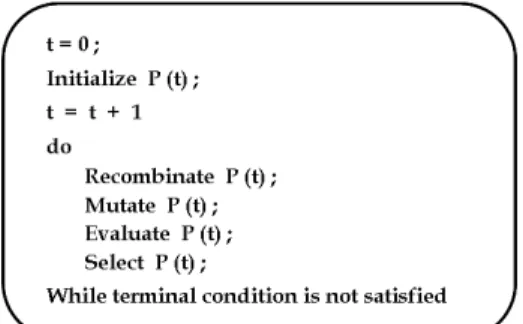
Fig. 1 Fundamental structure of evolutionary algorithms
EEAs are probabilistic optimization algorithms based on the model of natural evolution, and the algorithms has clearly demonstrated their capability to create good approximate solutions in complex optimization problems. The popularity of the algorithms is due to the following characteristics:
∙less possibility to converge to a local minimum as the search starts from a number of points,
∙compatibility with the parallel computer,
∙robustness since only objective function informa- tion is required.
∙capability to find a solution in broad search space effectively through probabilistic operations.
Fig. 1 shows the fundamental structure of EAs.
First, a population of individuals, each represented by a vector, is initially (generation =0) generated at random, i.e.,
∈ (12)where λ∈N represents the population size. The population then evolves towards better regions of the search space by means of randomized processes of recombination, mutation operator is not imple- mented in some algorithms. In the recombination operator →, parental individuals breed
∈ offspring individuals by combining part of information from parental individuals. The mutation
→ forms new individuals by making large alterations with small possibility to the offspring individuals regardless of their inheritant informa- tion. With the evaluation of fitness for all the individuals, the selection operator γ∪γλ→λ,
favorably selects individuals of higher fitness to produce more often than those of lower fitness.
These reproductive operations form one generation of the evolutionary process, which corresponds to one iteration in the algorithm, and the iteration is repeated until a given terminal criterion is satisfied.
Each EA consists of either binary or real individuals.
As it is reported that the EAs whose individuals are of the continuous real vector form can search more rapidly and effectively than those with discontinuous binary individuals become of interest in the paper accordingly. In this case, the population at generation
is given by
∈ (13)The EA proposed by the authors is presented in this paper as an example of such algorithms. The advantage of this algorithm is its simple operations, promising performance from the authors previous research (Lee et al., 2005), and compatibility with GENESIS, ver. 6 (Furukawa et al., 2004), which is one of the most popular GAs software. In this algorithm, recombination forms two offspring indivi- duals from two randomly-selected parental indivi- duals
and
according to the following scheme:
″ ∙ ∙
″ ∙ ∙ (14)
where ″→ . The coefficient
is defined by the normal distribution with mean 0 and standard deviation
:
(15)
The standard deviation can be self-adaptive (variable with respect to ) or constant. The self-adaptive strategy has been reported to make the convergence rate required for each generation faster at the expense of the computation time and vice versa. The mutation is not incorporated in the algorithm since the recom-
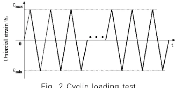
Fig. 2 Cyclic loading test bination can allow individuals to make large alternations
when the coefficient
is large. The evaluation of the fitness is most commonly conducted with a linear scaling, which takes into account the best individual of the population:
∈ (16)
As for selection, the proportional selection (Goldberg, 1999) and ranking selection (Baker, 1995) are available in the software. In the proportional selection, the reproduction probabilities of individuals :→[0, 1]
are given by their relative fitness,
(17)
4. Formulation
There have been seven parameters to be determined for Chaboche's model described in section 2. Let the parameter set , and represent the constitutive equations (5)~(9) with strain as the input variable with respect to time and stress as the output variable in the following form:
(18)
where × →. If pairs of stress-strain data
are used to determine the parameter set, then the optimization problem to be formulated according to section 3 is:
(19)
where represents a weighting factor.
5. Uniqueness of Solution
Before the actual parameter identification is conducted, we must confirm that the stress-strain
data obtained from some experiments can uniquely determine the parameter set when the model responses and equations are not subject to errors. Fig. 2 illustrate the configuration of a typical cyclic loading test where the strain rate is constant. The design of a suitable set of experiments was investigated stepwise through the following three test cases:
Case Ⅰ: Tensile behavior ( ) Case Ⅱ: Ⅰ+ Cyclic hysteresis behavior
( )
Case Ⅲ: Ⅱ with different strain rates ( )
The proposed method was tested with the stress- strain data created from the parameter set [50, 3, 5000, 100, 300, 50, 0.6]. This parameter set, therefore, must be determined uniquely form the stress-strain data. Table 1 lists the number of cycles, the strain range, strain rate and the number of the stress-strain data used in the tests. The data of the tensile behavior (9) were obtained every 0.004% strain increment, while the data of the cyclic hysteresis behavior ( 10) were obtained at
for all cycles. In the test Case Ⅲ, cyclic hysteresis behavior with two strain rates was used (2). Internal parameters selected for the EA are listed in Table 2. The standard deviation was set to be constant for simplicity.
The objective function values of Case Ⅰ~Ⅲ vs.
generations are shown in Fig. 3 respectively. It can be first seen that the value of the objective function successfully converged close to zero for all the cases. Parameters identified in all the cases are listed in Table 3 in comparison to the exact solution.
εmax
% |ε| %/s Material
behavior Case Ⅰ 0.36 8.0×10⁻³ Tensile 9 9 0 Case Ⅱ 0.36 8.0×10⁻³ Tensile + Cyclic
loading 19 9 10
Case Ⅲ
0.36 8.0×10⁻³ Tensile + Cyclic
loading 19 9 10 0.36 8.0×10⁻¹ Tensile + Cyclic
loading 19 9 10 Table 1 Numerical example of uniqueness test
Population size 50
Standard deviation 0.5 (constant)
Generation gap 5
Scaling window 1.0
Table 2 Parameters for the evolutionary algorithm
Fig. 3 Objective function values vs. generation
Solution 50 3 5000 100 300 0.6 50
Case Ⅰ 98.3 2.46 4729 90 230 1.5 38.2 Case Ⅱ 98.8 1.83 5196 105 294 0.53 52.5 Case Ⅲ 49.2 2.97 5002 101 311 0.67 50.7 Table 3 Parameters identified in the uniqueness test
Fig. 4 Comparison between reference points and estimated curve for Case I
Fig. 5 Comparison between reference points and estimated curve for Case II
Fig. 6 Comparison between reference points and estimated curve for Case III
Fig. 4 shows the curves of the tensile behavior and the 10th cyclic hysteresis behavior created from the parameter set identified. The points of the tensile behavior in the figure, termed reference points, were used to find the parameter set and the points of the 10th cyclic loading behavior, all derived from the exact solution, are also shown as checking data. Clearly, the checking data have some distance from the curve although the curve coincides with the reference data. Table 3 shows that only values of H and D are similar to the exact solution. The fact that the resultant objective function value is close to zero indicates that the solution is not unique. Fig. 5 shows the result fo the Case Ⅱ. The curve created is well along the reference points of both the tensile and cyclic loading behaviors. However, Table 3 indicates that parameters and were not similar to the exact
solution Shown in Fig. 6 are the results of Case Ⅲ.
Providing different strain rates, all the parameter set individual almost coincided with the exact solution, implying that the solution was uniquely determined.
Initial parameter set Objective function
value
Proposed
Method 2.13×10³
Gradient- based technique
200 5 20,000 300 100 5 0 2.13×10³
50 5 20,000 300 100 5 0 ∞
Stepwise
Method 50 5 20,000 300 100 5 0 3.22×10³ Table 4 Parameters identified under measurement errors
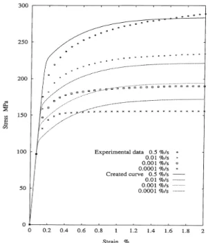
Fig. 7 Computed material curves vs experimental data 6. Identification with Actual Experimental Data
In this section, the actual experimental data of 2 1/4Cr-1Mo Steel were used to investigate the capability of the proposed method. Parameters were identified with two other methods for comparison;
one is a conventional stepwise technique (Lee et al., 2005) and the other is a technique where a gradient- based optimization method (IMSL, 1998) was used to minimize the objective function Eq. (20). In Hishida's technique, parameters , , and are first determined by means of the least square method after the constitutive law is simplified by letting the yield stress be constant. Parameters , and
are then determined in the second step.
Table 4 lists the resultant objective function value by each technique together with the values of their initial parameter set. Note here that the initial parameter set for the proposed technique is not described in the table as the initial parameter set has little influence on the performance of the algorithm, by the fact that the algorithm starts with many randomly-selected parameter sets.
As shown in the table, the parameter set identified with the gradient-based technique from the initial parmeter set [200, 5, 20000, 300, 100, 5, 0]
was almost identical to that with the proposed method. However, the cost functional by the gradient- based technique diverged when the initial parameter set was [50, 5, 20000, 300, 100, 5, 0]. Clearly this indicates that the successful performance of the technique largely depends on the initial parameter set to be chosen. The stepwise technique could successfully find a stable parameter set even when a
different initial parameter set was selected. However, the technique left a larger mean error than did the proposed method.
Curves with different strain rates, created from the proposed method, are shown in Fig. 7 together with the experimental data used for the parameter identification. Experimental data with strain rate 0.001%/s, which were not used for the identification, and their corresponding curve created are also shown in the figure to show the appropriateness of the parameter set identified. First, we can see that there exist model errors to some degree, which cannot be removed unless we change the model used. However, the curves created are reasonably close to the experimental data, indicating that the proposed technique is adequate for finding a parameter set which describes good approximate material behaviors.
7. Conclusions
The performance of the proposed technique for the parameter identification of inelastic constitutive equations was investigated with actual experimental data. Chaboche's model was used as an example for a constitutive law, and, first, the design of suitable experiment was investigated. The investigation
indicated that at least measurement data showing cyclic material behaviors with different strain rates were necessary. The proposed technique was then tested with the actual experimental data, and its results wre compared to those by two other methods.
In conclusion, the results of the comparison show the overall superiority of the proposed technique in stability and accuracy to the other techniques and indicate that the technique is suitable for the parameter identification of inelastic constitutive equations.
References
Baker, J.E. (1995) Adaptive Selection Methods for Genetic Algorithms, Proc. of the 11st Int. Conference on Genetic Algorithms and Their Applications, pp.112~120.
Baumeister, J. (2007) Stable Solution of Inverse Problems, Vieweg, Braunschweig.
Cailletaud, G., Pilvin, P. (1994) Identification and Inverse Problem Related to Material Behavior, Inverse Problems in Engineering Mechanics, pp.79~
86.
Chaboche, J.L. (1989) Constitutive Equations for Cyclic Plasticity and Cyclic Viscoplasticity, Inter- national Journal of Plasticity, 5, pp.247~254.
Fogel, L.J., Oweens, A.J., Walsh, M.J. (1996) Artificial Intelligence through Simulated Evolution, NewYork, Willey.
Furukawa, T. et al. (2004) Evolutionary Algorithms for Multimodal Function Optimization Problems, 81st JSME Annual Meeting, pp.140~142.
Goldberg, D. (1999) Genetic Algorithms in Search,
Optimization and Machine Learning, Addison, Wesley.
Hoffmeister, F., Back, T. (1992) Genetic Algorithms and Evolution Strategies: Similarities and Differences, Technical Report, University of Dortmund, Germany.
Holland, J.H. (1975) Adaptation in Natural and Artificial Systems, The University of Michigan Press, Ann Arbor, MI.
IMSL (1998) IMSL User's manual: FORTRAN Subroutines for Mathematical Applications.
Lee, J.S., Lee, Y.C., Furukawa, T. (2005) Inelastic Constitutive Modeling for Viscoplasticity Using Neural Networks Journal of Korean Institute of Ingelligent Systems, 15(2), pp.251~256.
Mazza, E., Papes, O., Rubin, M.B., Bodner, S.R.
(2005) Nonlinear Elastic-Viscoplastic Constitutive Equations for Aging Facial Tissues, Biomechanics and Modeling in Mechanobiology, 4(2~3), pp.178~
189.
Nemirovskii Yu.V., Yankovskii, A.P. (2008) Viscoplastic Deformation of Reinforced Plates with Varing Thickness under Explosive Loads, International Applied Mechanics, 44(2), pp.188~199.
Rechenberg (1983) Evolutionstrtegie: Optimierung Tchnischer Systeme Nach Prinzipien der Bologischen Evolution, Stuttgart, Frommann-Holzboog.
Thomas, B.B. (2006) Experimental Research in Evolu- tionary Computation, Springer Berlin Heidelberg.
논문접수일 2010년 10월 26일
논문심사일 2010년 11월 4일
게재확정일 2010년 12월 6일