A Flexible Modeling Approach for Current Status Survival Data via Pseudo-Observations

A Flexible Modeling Approach for Current Status Survival Data via Pseudo-Observations

Seungbong Han ¹ · Adin-Cristian Andrei ² · Kam-Wah Tsui ³

1

Department of Clinical Epidemiology and Biostatistics, Asan Medical Center, University of Ulsan College of Medicine;

BCVI Clinical Trials Unit, Feinberg School of Medicine, Northwestern University

3

Department of Statistics, University of Wisconsin-Madison

(Received September 27, 2012; Revised October 22, 2012; Accepted November 13, 2012)

Abstract

When modeling event times in biomedical studies, the outcome might be incompletely observed. In this paper, we assume that the outcome is recorded as current status failure time data. Despite well-developed literature the routine practical use of many current status data modeling methods remains infrequent due to the lack of specialized statistical software, the difficulty to assess model goodness-of-fit, as well as the possible loss of information caused by covariate grouping or discretization. We propose a model based on pseudo-observations that is convenient to implement and that allows for flexibility in the choice of the out- come. Parameter estimates are obtained based on generalized estimating equations. Examples from studies in bile duct hyperplasia and breast cancer in conjunction with simulated data illustrate the practical advan- tages of this model.

Keywords: Breast cancer, current status data, generalized estimating equations, NPMLE, regression model.

1. Introduction

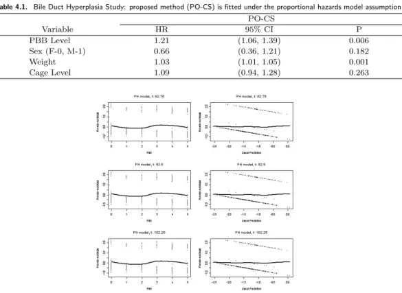
Current status data are obtained when the event time of interest T is solely known to precede or to succeed the examination time C. Examples arise in numerous settings that include studies on epidemiology (Namata et al., 2007), demography (Diamond et al., 1986; Grummer-Strawn, 1993), cardiovascular disease (Wang and Ding, 2000), or animal carcinogenicity (Tong et al., 2007). For instance, in the rat tumorigenicity experiment described by Dinse and Lagakos (1983) and Ghosh (2003), of interest was the relationship between the level of polybrominated biphenyl mixture(PBB) and the presence of bile duct hyperplasia(BDH). However, the BDH presence could be only known at the time of natural death or intentional sacrifice. Therefore, the obtained data type is the current status format. As an another example, a Phase III Breast Cancer Trial (IBCSG, 1996) was Andrei is partially supported by NIH grants P30 CA014520-33 and UL1 RR025011. Tsui is supported in part by the NSF grant DMS-0604931.

1

Corresponding author: Research Professor, Department of Clinical Epidemiology and Biostatistics, Univer-

sity of Ulsan College of Medicine, Asan Medical Center, 86 Asanbyeongwon-gil, Songpa-gu, Seoul 138-736,

Korea. E-mail: [email protected]

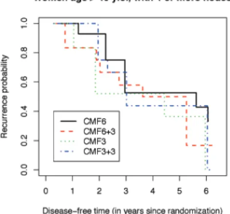
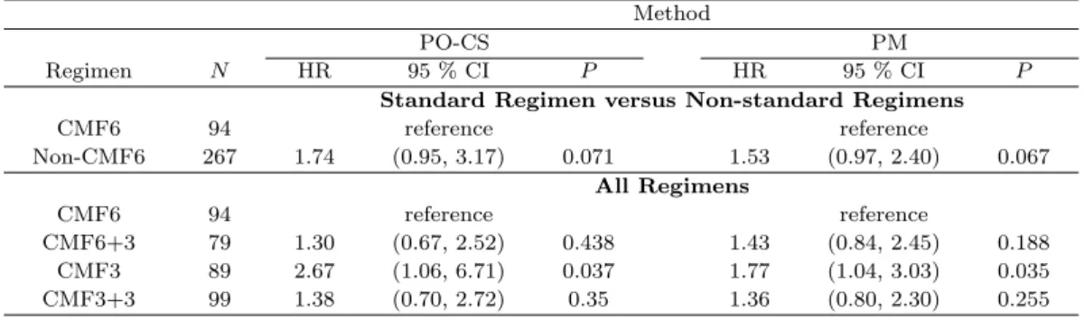
conducted to determine the optimal duration and timing of a cyclophosphamide, methotrexate and fluorouracil(CMF) combination chemotherapy in relationship to disease-free survival(DFS). When the patient DFS status is assessed at a six-year post enrollment (or at the most recent clinic visit), the outcome is recorded in current status format. Scientific questions such as risk factor findings and prognostic model buildings could be appropriately addressed via regression modeling. For current status data outcomes, important contributions have been made under several structural models that include: (i) proportional hazards (Huang, 1996); (ii) proportional odds (Dinse and Lagakos, 1983; Huang, 1995; Rossini and Tsiatis, 1996; Huang and Rossini, 1997); (iii) linear transformation (Shen, 2000; Sun and Sun, 2005; Tian and Cai, 2006) or (iv) additive-risk (Lin et al., 1998; Shiboski, 1998; Martinussen and Scheike, 2002). Despite the progression made, many existing methods are not routinely used in practice for a variety of reasons, such as: (a) a pervasive lack of software availability, amplified by a non-trivial implementational effort; (b) difficulty/impossibility to be extended to contexts that require different structural assumptions (for example, a method developed under proportional hazards might not be translated to proportional odds scenarios);

(c) inherent non-convergence or local convergence issues associated with EM-type algorithms; (d) unwarranted assumptions imposed on the data, such as covariate grouping or discretization; and (e) lack of convenient model diagnosis and goodness-of-fit tools. We propose a semiparametric regression approach based on the jackknife pseudo-observations(POs) (Tukey, 1958). This technique has been used with right-censored data to model transition probabilities in multi-state models (Andersen et al., 2003), restricted mean survival times (Andersen et al., 2004), cumulative incidence functions in competing risks (Klein and Andersen, 2005; Logan et al., 2011), quality-of-life-adjusted survival (Andrei and Murray, 2007), survivorship with crossing survival curves (Logan et al., 2008).

Andersen and Perme (2010) provide a useful review. Recently, Han et al. (2012) have extended the POs technique to interval-censored data; however, the use of pseudo-observations in current-status data problems has not yet been explored and constitutes the main theme of this paper. There are several advantages to this approach:

• Inference could be carried out via generalized linear models/generalized estimating equations.

• Algorithm-convergence problems are avoided.

• Practical implementation in major statistical software packages is straightforward and requires minimal programming.

The rest of this paper is organized as follows. Section 2 presents methodological developments.

Section 3 shows the simulation results indicating excellent method performance. In Section 4, we present detailed analyses of the animal carcinogenicity study (Dinse and Lagakos, 1983) and the Phase III Breast Cancer Trial (IBCSG, 1996). In the discussion section, we make additional remarks and draw conclusions.

2. Pseudo-Observation-Based Regression

Let independent T

and C

be the event time of interest and the examination time for subject i,

respectively, where i = 1, . . . , n. The current status data consist of {(C

, δ

); i = 1, . . . , n}, where

δ

= I(T

≤ C

). If δ

= 1, then T

is left-censored; otherwise, it is right-censored. Let Z

be a

p-dimensional baseline covariate vector for subject i. Denote S(t |Z

) = P (T

> t |Z

) to be the

conditional survival function of T

and α(t) to be a function of time. Assume that the underlying

model is

g{S(t|Z

)} = α(t) + β

Z

, (2.1)

where β is the covariate effect vector and g(·) is a smooth link function. For instance, g(s) = log[− log(s)] (0 < s < 1) leads to the proportional hazards model and g(s) = log(s/(1 − s)) (0 <

s < 1) induces the proportional odds model, while the probit link function yields the probit model.

2.1. Pseudo-observations for current status data

Suppose that ˆ S(t) is a consistent nonparametric estimator of the marginal survival function S(t) = P (T

> t) based on {(C

, δ

), i = 1, . . . , n }. Similarly, ˆ S

(t) denotes the corresponding version of the estimator computed based on the reduced sample {(C

, δ

), j ̸= i}, where i = 1, . . . , n. Andersen et al. (2003) originally defined the i

pseudo-observation as η

= n ˆ S(t) − (n − 1) ˆ S

(t). However, we define the i

pseudo-observation as

ν

= ng { S(t) ˆ

} − (n − 1)g { S ˆ

(t)

}

, (2.2)

where t > 0 is such that 0 < min { ˆ S(t), ˆ S

(t); i = 1, . . . , n } < 1. This definition differs slightly from the one defined by Andersen et al. (2003) in that it incorporates the link function g( ·). This way, the occurrence of out of range probability estimates is avoided. We subsequently compare our newly- defined PO approach with the original PO approach suggested by Andersen et al. (2003). We first describe an existing method to obtain the nonparametric maximum likelihood estimator(NPMLE).

As such, define {s

}

to be the increasingly ordered, unique elements of {0, C

, . . . , C

} and recall that δ

= I(T

≤ C

). Let n

= ∑

i=1

I(C

= s

) and r

= ∑

i=1

δ

I(C

= s

) be the number of individuals observed at time s

and the number who have failed prior to s

among those who were observed at s

, respectively. The likelihood function is

L(s) =

∏

[1 − S(s

)]

[S(s

)]

, (2.3)

where s = {s

, . . . , s

}. Clearly, an estimator ˆ S(t) of S(t) is determined up to the values at unique censoring times. Using isotonic regression methods, Robertson et al. (1988) showed that the maximization of L(s) subject to the monotonicity constraint S(s

) ≥ · · · ≥ S(s

) is equivalent to the minimization of

∑

n

[ r

n

− 1 + S(s

) ]

. (2.4)

By using the max-min formula, one can obtain a closed-form NPMLE of S as

S(s ˆ

) = 1 − max

u≤j

 

 

 

 min

v≥j

∑

r

∑

n

 

 

 



. (2.5)

2.2. Parameter estimation

To fit model (2.1), one may proceed as follows: instead of regressing g{S(t|Z

)} on Z

, one can regress

ν

on Z

. In doing so, the pseudo-observation ν

serves as a substitute for the response g {S(t|Z

) }.

This approach has also been taken by Han et al. (2012) to model interval-censored survival data.

This approach is legitimized by the fact that the POs thus obtained are nearly independent (Tukey, 1958; Andersen et al., 2004). Note that the POs ν

were obtained at a single time point t.

However, parameter estimates efficiency could be markedly improved when POs are computed at multiple timepoints t

< · · · < t

, where t

> A = inf {t : min{ ˆ S(t), ˆ S

(t); i = 1, . . . , n } > 0} and t

< B = sup {t : max{ ˆ S(t), ˆ S

(t); i = 1, . . . , n } < 1}. Let ν

= (ν

, ν

, . . . , ν

)

be the PO vector thus obtained. Define γ = (β, α(t

), . . . , α(t

))

and µ

= (α(t

)+β

Z

, . . . , α(t

)+β

Z

)

. Let U

(γ) be (∂µ

/∂γ)

V

(ν

− µ

). Estimates ˆ γ for γ are obtained based on the following generalized estimating equations:

U (γ) =

∑

U

(γ) =

∑

( ∂µ

∂γ )

V

(ν

− µ

) = 0, (2.6) where V

is the working covariance matrix for ν

. Under standard regularity conditions, it fol- lows that √

n(ˆ γ − γ) is asymptotically normal with mean zero and covariance matrix that can be consistently estimated by the following sandwich estimator,

Var(ˆ d γ) = { I(ˆ γ)

}

c

var {U(ˆγ)} { I(ˆ γ)

}

, (2.7)

where I(γ) = ∑

i=1

Z

V

Z

and var c {U(ˆγ)} = ∑

i=1

U

(ˆ γ)U

(ˆ γ)

. Alternatively, one may use jackknife variance estimators such as the one-step or the approximate procedures proposed by Yan and Fine (2004). For GEE implementation in practice, one may use the R function geese from the package geepack (Yan, 2002) or the function gee from the package gee (Vincent, 2011) in R.

However, one can use the P roc Genmode procedure in SAS. In the following simulation section, we compare the proposed method with existing approaches and investigate the impact of incorporating the link function for the PO construction (denoted by PO-CS : ν

) by comparing it with the original PO approach (denoted by PO-CS : η

).

3. Simulation Studies

We apply the proposed approach to data generated from: (1) a proportional hazards, (2) propor- tional odds. Samples of size n = 200 and 300 are considered and each scenario is replicated 1, 000 times. Throughout, POs are obtained at 10 or 25 equally-spaced time points between the 20

and the 80

percentiles of the ordered unique elements of the set {0, C

: i = 1, . . . , n }. A first-order autoregressive working correlation matrix V

is assumed. In all simulation scenarios, 3-dimensional covariates Z

= (Z

, Z

, Z

)

with independent entries are generated.

3.1. A proportional hazards model

This model is of the form

log [ − log {S(t|Z)}] = log {∫

0

h

(u)du }

+ β

Z, (3.1)

where h

(·) is the baseline hazard function. The corresponding link function is g(s) = log{− log(s)}.

We consider the baseline hazard function h

(t) = 1, while Z

, Z

and Z

are generated from U (1, 2), N (0, 1) and Bernoulli(0.5) distributions, respectively and (β

, β

, β

) = (−0.5, 0.5, −0.5).

Monitoring (current status assessment) times C

are generated from a uniform U (1, 3) distribution.

We compare the proposed PO-CS method using the ν

with the η

-based PO method. PO-CS

Table 3.1. Proportional hazards model: ˆ β

= empirical mean of estimated β

values, SE(β

) = empirical mean of estimated standard errors for ˆ β

, ESE = empirical standard error for ˆ β

, CP = coverage probability of true β

by the 95% confidence intervals for i = 1, 2 and 3, For var( ˆ c β), the sandwich estimator(SA) in (7) or approximate jackknife(AJ) variance estimate(VE) is used. ν

and η

represent incorporating the link function for the PO-construction and the original i

PO proposed by Anderson et al. (2003), respectively. ⋆ means numbers are > 10

.

n = 200 β

= −0.5 β

= 0.5 β

= −0.5

Method J VE β ˆ

SE ESE CP β ˆ

SE ESE CP β ˆ

SE ESE CP

PO-CS : ν

25 SA −0.47 0.40 0.41 0.93 0.46 0.11 0.11 0.92 −0.47 0.23 0.23 0.94 PO-CS : ν

25 AJ −0.45 0.39 0.37 0.97 0.47 0.11 0.12 0.91 −0.49 0.22 0.22 0.98 PO-CS : ν

10 AJ −0.45 0.41 0.37 0.98 0.47 0.11 0.12 0.93 −0.49 0.24 0.22 0.98 PO-CS : η

25 AJ −17.9 ⋆ 227 0.66 1.67 ⋆ 35.1 0.05 −6.89 ⋆ 101 0.24 PO-CS : η

10 AJ −0.64 0.66 2.13 0.87 0.68 0.23 0.51 0.91 −0.69 0.38 1.05 0.84 PM −0.55 0.42 0.43 0.97 0.54 0.18 0.19 0.94 −0.52 0.27 0.26 0.96

n = 300 β

= −0.5 β

= 0.5 β

= −0.5

Method J VE β ˆ

SE ESE CP β ˆ

SE ESE CP β ˆ

SE ESE CP

PO-CS : ν

25 SA −0.48 0.32 0.33 0.94 0.47 0.09 0.09 0.93 −0.47 0.19 0.19 0.94 PO-CS : ν

25 AJ −0.48 0.35 0.36 0.97 0.47 0.09 0.10 0.91 −0.46 0.19 0.20 0.95 PO-CS : ν

10 AJ −0.48 0.36 0.37 0.95 0.47 0.10 0.11 0.92 −0.48 0.21 0.23 0.95 PO-CS : η

25 AJ −0.65 0.57 0.97 0.87 0.63 0.19 0.38 0.88 −0.57 0.31 0.42 0.90 PO-CS : η

10 AJ −0.54 0.43 0.48 0.91 0.58 0.15 0.20 0.92 −0.54 0.25 0.28 0.91 PM −0.53 0.32 0.34 0.96 0.53 0.14 0.15 0.95 −0.52 0.20 0.21 0.96

(η

) uses a complementary log-log link function g(s) = log(− log(1 − s)) in the geese routine.

Currently, the desired log(− log(s)) link function is not available in the geese function. While we use approximate jackknife(AJ) variance estimate for var( ˆ c β), we also try the sandwich estimator(SA) as an alternative (J = 25 case). To compare with an existing method, a parametric Weibull method (PM) is considered using the function survreg based on the package survival in R. Table 3.1 shows simulation summary results and it includes the empirical mean of the ˆ β estimates, the mean of the estimated standard errors for ˆ β (SE), the empirical standard error for β (ESE), the coverage probability(CP) of the true β by the 95% confidence intervals. Overall, PO- ˆ CS (ν

) produces coefficient estimates that are very close to true values, while the corresponding 95% confidence intervals exhibit appropriate coverage probabilities. As the sample size increases, we obtain more efficient paramater estimates. No matter what variance estimates are used, these findings are not changed. However, if we use the original PO approach based on η

(PO-CS : η

) and the complementary log-log link function in the geese routine, we end up with severely biased coefficient estimates and quite unstable variance estimates. Although the bias slightly decreases as the sample size increases, its SE and ESE are significantly worse compared to PO-CS (ν

). Note that the parametric model(PM) performs reasonably well, as expected. Surprisingly, the efficiency of PO-CS (ν

) is as good as PM although our method does not assume any specific distribution.

Average per simulation run-time for the PO based methods was about 2 minutes and 8 minutes for n = 200 and 300, respectively.

3.2. A proportional odds model

The second simulation set is devised for the proportional odds model logit {S(t|Z)} = logit {S

(t) } − β

Z,

with baseline survival function S

(t). In this model, positive β represents a hazardous effect on the

Table 3.2. Proportional odds model: ˆ β

= empirical mean of estimated β

values, SE(β

) = empirical mean of estimated standard errors for ˆ β

, ESE = empirical standard error for ˆ β

, CP = coverage probability of true β

by the 95% confidence intervals for i = 1, 2 and 3, For var( ˆ c β), the sandwich estimator(SA) in (7) or approximate jackknife(AJ) variance estimate(VE) is used. ν

and η

represent incorporating the link function for the PO-construction and the original i

PO proposed by Anderson et al. (2003), respectively. ⋆ and † mean numbers are > 10

or < −10

n = 200 β

= −0.5 β

= 0.5 β

= −0.5

Method J VE β ˆ

SE ESE CP β ˆ

SE ESE CP β ˆ

SE ESE CP

PO-CS : ν

25 SA −0.49 0.32 0.34 0.93 0.48 0.16 0.17 0.92 −0.55 0.32 0.35 0.92 PO-CS : ν

25 AJ −0.49 0.33 0.35 0.96 0.48 0.15 0.16 0.93 −0.54 0.32 0.33 0.95 PO-CS : ν

10 AJ −0.50 0.34 0.35 0.94 0.48 0.17 0.18 0.94 −0.54 0.34 0.36 0.95 PO-CS : η

25 AJ −158 2.26 1821 0.84 0.81 0.69 2.83 0.86 118 2.8 1838 0.85 PO-CS : η

10 AJ −0.60 0.44 0.55 0.92 0.61 0.25 0.33 0.92 −0.65 0.44 0.55 0.91 PM −0.36 0.24 0.23 0.87 0.35 0.15 0.16 0.68 −0.37 0.24 0.24 0.84

n = 300 β

= −0.5 β

= 0.5 β

= −0.5

Method J VE β ˆ

SE ESE CP β ˆ

SE ESE CP β ˆ

SE ESE CP

PO-CS : ν

25 SA −0.50 0.27 0.27 0.95 0.47 0.13 0.14 0.95 −0.46 0.27 0.27 0.95 PO-CS : ν

25 AJ −0.50 0.26 0.28 0.96 0.48 0.12 0.13 0.95 −0.47 0.25 0.26 0.95 PO-CS : ν

10 AJ −0.50 0.29 0.29 0.96 0.47 0.14 0.14 0.95 −0.45 0.28 0.28 0.96

PO-CS : η

25 AJ † ⋆ ⋆ 0.31 ⋆ ⋆ ⋆ 0.06 † ⋆ ⋆ 0.28

PO-CS : η

10 AJ † ⋆ ⋆ 0.95 ⋆ ⋆ ⋆ 0.96 † ⋆ ⋆ 0.95

PM −0.36 0.19 0.23 0.77 0.33 0.12 0.16 0.52 −0.33 0.19 0.19 0.77

survival. We consider S

(t) = e

. Z

, Z

and Z

are generated from Bernoulli(0.5), N (0, 1) and Bernoulli(0.5) distributions, respectively and regression coefficients (β

, β

, β

) are fixed at ( −0.5, 0.5, −0.5). As in the proportional hazards model, the monitoring times C

are generated from a uniform distribution using survival time T . The appropriate link function is g(s) = logit(s).

For comparison, we also employ a parametric method assuming logistic distribution obeying a proportional odds model. The results shown in Table 3.2, indicate that the proposed PO-CS (ν

) performs very well in terms of bias and coverage probabilities. One can also observe PO-CS (η

) produces severely biased and unstable results even in n = 300. The poor performance of the PO-CS (η

) may be due to many occurrences POs out of the (0, 1) range. However, the PM appears to overestimate the covariate effects and CPs quite below the nominal level 95%.

3.3. Model assessment

Recently, Perme and Anderson (2008) suggest a graphical method for goodness-of-fit based on

pseudo-observations. Following their approach, a raw residual (at each time point) can be defined by

ν

−[ˆα(t)+ ˆ β

Z

]. Then its standardized pseudo-residual can be defined as [ν

− {ˆα(t) + ˆ β

Z

}]/Ψ,

where Ψ is an empirical standard error for the raw residuals; subsequently, we use these residuals

as a graphical diagnostic tool to evaluate a model fit. Suppose that survival times T

are gener-

ated from the proportional hazards(PH) model and model fitting is conducted based on the PH

assumption. In Figure 3.1, the standardized pseudo-residuals from the simulated proportional haz-

ards model (n = 300, J = 25 and AJ variance estimate) are plotted against each covariate vector

and its linear predictor ˆ α(t) + ˆ β

Z

. Although we can compute the pseudo-residuals at each time

point, we may select three time points which are chosen at three quartiles (Q

, Q

, Q

) based on the

estimated survival function. To detect any trend, we may add a curve showing a smooth average

through the residuals. Based on the smoother there seems no trend to indicate the proportional

hazards assumption violation.

Figure 3.1. Goodness-of-fit for the proportional hazards(PH) regression based on pseudo-residuals. Survival times T

are generated from the PH model and model fitting is conducted based on PH assumption. Each row presents one of the three time points chosen and each column presents one of the three variables and its linear predictor.

4. Examples

4.1. The Bile Duct Hyperplasia Study

We apply the proposed method PO-CS (based on ν

) to the bile duct hyperplasia study (Dinse

and Lagakos, 1983) mentioned in the Introduction. The scientific goal of this study is to investi-

gate the association between polybrominated biphenyl mixture(PBB) and the presence of bile duct

hyperplasia(BDH) at the examination time. Over a 6-month period, researchers administered 125

oral doses of PBB to 319 Fisher rats. Current status data are obtained as bile duct hyperplasia

occurrence could only be established at the time of natural death or intentional sacrifice. Besides

the PBB level (on a 0-5 scale) outcome, the following variables are collected: sex (0-female, 1-male),

baseline weight (in grams) and cage level (1-top, . . . , 5-bottom). As in Dinse and Lagakos (1983)

and Tian and Cai (2006), we assume that both PBB and cage level are continuously-distributed

random variables. In addition, we assume that time-to-bile duct hyperplasia development follows

a proportional hazards model. Pseudo-observations have been obtained at 25 equally-spaced time

points chosen as described in the previous section. Analysis results in Table 4.1 present an esti-

mated covariate hazard ratio(HR), corresponding 95% confidence interval and p-value(P ). Using

the proposed PO-CS method, the PBB dose estimated HR is 1.21 (P = 0.006), indicating that a

one-unit increase in the PBB dose level is associated with a 20% increase in the risk of developing

BDH. The model also indicates that a higher weight is also significantly associated with a 3% in-

Table 4.1. Bile Duct Hyperplasia Study: proposed method (PO-CS) is fitted under the proportional hazards model assumption.

PO-CS

Variable HR 95% CI P

PBB Level 1.21 (1.06, 1.39) 0.006

Sex (F-0, M-1) 0.66 (0.36, 1.21) 0.182

Weight 1.03 (1.01, 1.05) 0.001

Cage Level 1.09 (0.94, 1.28) 0.263

Figure 4.1. Bile Duct Hyperplasia Study: goodness-of-fit for the proportional hazards regression model based on pseudo-residuals.

crease in the BDH occurrence risk (HR = 1.03, 95% CI = (1.01, 1.05)). The parametric model(PM) has encountered convergence problems and no HR estimates are obtained. A possible explanation might be that by employing EM-type algorithms to estimate covariate effects, one might face diffi- culties such as non-convergence or local convergence. A built-in feature of the proposed PO-based regression method is that it avoids such convergence issues. It is worth mentioning that Dinse and Lagakos (1983) could not establish a statistically significant PBB dose level effect.

Figure 4.1 shows plot of the pseudo-residuals against PBB and linear predictor in the model at time points 82.75, 92.5, and 102.25. The smooth curve seems to vary around 0 with no systematic trends so the proportional hazards assumption is reasonable.

4.2. The IBCSG Trial VI Study

We further illustrate the proposed PO-CS regression method using the International Breast Can-

cer Study Group(IBCSG) Trial VI (IBCSG, 1996) data. This trial has investigated the optimal

duration and timing of a 12-month postoperative combination chemotherapy of cyclophosphamide,

methotrexate and fluorouracil(CMF). Of interest was how CMF, with or without subsequent re-

introduction, is associated with time to breast cancer recurrence. Between July 1986 to April 1993,

eligible patients were randomly assigned (with equal probability) to one of the following four regi-

mens: (i) CMF for six initial consecutive courses on months 1–6 (CMF6); (ii) CMF for six initial

consecutive courses on months 1–6 plus three single courses of re-introduction CMF given on months

Figure 4.2. IBCSG Trial VI: time to breast cancer recurrence estimates in the four regimens for women with four or more nodes, age > 40 years at baseline.

9, 12, 15 (CMF6+3); (iii) CMF for three initial consecutive courses on month 1–3 (CMF3) and (iv) CMF for three initial consecutive courses on months 1–3 plus three single courses of re-introduction CMF given on months 6, 9, 12 (CMF3+3). Based on repeated clinic visits, the cancer recurrence time was assessed as the difference between the randomization date and the relapse date, defined as the visit when the cancer relapse was established. For illustrative purposes, we have obtained a current status data structure as follows: for a patient, their observation time C was set at 6 years after randomization. At the observation time, we constructed the censoring indictor δ for each individual based on the disease progression date D. If D ≤ C, δ = 1, otherwise δ = 0. However, about a quarter of patients did not experience disease progression during follow-up. In this case, if C is less than the patient’s last clinic visit date, then δ is set to 0. However, when C is greater than the patient’s last clinic visit date, we change the observation time into the patient’s last clinic visit date and set δ to 0, assuming no disease-progression up to the last clinic visit.

We carried out two sets of analyses: (1) first, we have compared the standard regimen (CMF6) vs.

the non-standard regimens combined (CMF6+3, CMF3 and CMF3+3); (2) next, we compared all four regimens: CMF6, CMF6+3, CMF3, and CMF3+3. Patient age at baseline and node group status are known predictors of disease free survival(DFS) time (IBCSG, 1996; Gruber et al., 2008).

Therefore, in this example, we focus attention on a high-risk group of 361 women that are 40 years or older at baseline and have four or more cancer nodes. Figure 4.2 suggests that patients receiving CMF3 experience increased mortality compared to those receiving the standard CMF6.

Besides, non-standard regimens appear to be associated with an increased risk of recurrence and regression models assuming a proportional hazards underlying structure were constructed to test the statistical significance of these trends. As in the simulation study, POs have been calculated on a grid of 25 equally-spaced time points. Adjustment factors in the model were: tumor grade (1 (reduced), 2, 3 (increased)), tumor size ( ≤ 2 vs. > 2 cm across), vessel invasion (yes/no), estrogen receptor(ER) status (negative/positive) and progesterone receptor(PR) status (negative/positive).

Results shown in Table 4.2 include hazard ratio(HR) estimates, corresponding 95% confidence

intervals and p-values(P ). For comparison purposes, we also present the analysis results based on

the parametric method(PM) that assumes a Weibull distribution. Analyses employing the PO-

CS method reveal some interesting findings. First, when comparing standard vs. non-standard

Table 4.2. The IBCSG Trial VI example: regression models using PO-CS and PM under the proportional hazards assumption.

The number of patients receiving each regimen (N ) is included.

Method

PO-CS PM

Regimen N HR 95 % CI P HR 95 % CI P

Standard Regimen versus Non-standard Regimens

CMF6 94 reference reference

Non-CMF6 267 1.74 (0.95, 3.17) 0.071 1.53 (0.97, 2.40) 0.067

All Regimens

CMF6 94 reference reference

CMF6+3 79 1.30 (0.67, 2.52) 0.438 1.43 (0.84, 2.45) 0.188

CMF3 89 2.67 (1.06, 6.71) 0.037 1.77 (1.04, 3.03) 0.035

CMF3+3 99 1.38 (0.70, 2.72) 0.35 1.36 (0.80, 2.30) 0.255

regimens, the hazard rate in the non-standard group is almost twice as high as that of the standard regimen (HR = 1.74, 95% CI = (0.95, 3.17)), yet this falls short of statistical significance at the 5% α level (p-value = 0.071). The parametric method(PM) yields a HR = 1.53 and a p-value of 0.067. When comparing all four regimens, we find that mortality in the CMF3 arm is significantly higher than in the CMF6 (reference) group (p-value = 0.037 by PO-CS), with an estimated HR of 2.7. PM confirms this trend, producing hazard ratio 95% confidence intervals that do not contain 1. Based on the plot of the pseudo-residuals against the linear predictor in the model at time points 2.63, 3.41, and 4.18, the smooth curve seems to vary around 0 with no systematic trends (figure not shown here). Therefore we conclude that the proportional hazards assumption is satisfied.

5. Discussion

In this paper we develop a pseudo-observations-based regression method for current status data.

There is a close relationship with the causal inference approach of Chen and Tsiatis (2001) to obtain a marginal estimator of the τ restricted mean E[T ∧ τ], they require a conditional regression model and then average over the individuals in the sample. In our regression approach, the order of these steps is reversed; one first requires a marginal estimator of the quantity to be modeled, based on POs that serve as outcome substitutes become immediately available. The availability of the marginal survival function NPMLE and built-in software for generalized estimating equations enable testing and confidence intervals construction easily. As the implementational effort is minimal, there is potential for rapid applicability to biomedical studies involving current status data. In addition, the proposed semiparametric method is very flexible such that it can be extended to various models. Based on extra simulation results for the accelerated failure time model setting, the proposed PO-CS method produced reliable coefficient estimates with acceptable coverage probabilities. We also provide a graphical model assessment method to examine the regression model assumption using the standardized pseudo-residuals. By incorporating the link function into the PO-construction, we obtain more stable and less biased covariate effect estimates.

The choice of functional used for POs does not affect the performance of the proposed method.

Besides, this approach is more robust on the change of the number of time points in contrast with

most earlier work on pseudo-observations. When constructing pseudo-observations, the positioning

of the time points appears to matter. We may have more stable survival function estimates around

the median survival time. The choice of early and late time points can yield unstable POs. In this

paper, the positioning is determined based on the percentiles of observed observation time points.

Moreover, the number of time points may influence the efficiency of the coefficient estimates; as the number of time points increases, the efficiency of covariate effect estimate increases. In light of the extensive simulation studies, one may use 25 time points. All of the subsequent analyses for the example are conducted based on 25 time points. For the type of working correlation matrix, the first-order autoregressive working correlation matrix is used. Choosing another correlation structure such as independence seems to have no important effect for the parameter estimation; in addition, both the sandwich and the approximate jackknife variance estimates work reasonably well. Graw et al. (2009) provide the mathematical basis using influence functions and compact differentiability for the PO usage for the right-censored data. We plan to investigate the theoretical basis for the PO usage for the current status data, as well as the applicability of several model selection approaches (e.g., Hjort and Claeskens, 2008) to the current status data setting. So far, developments in this direction include the works of Ghosh (2003) for additive-risk models and Koul and Yi (2006) in a parametric setting. To conclude, the pseudo-observations-based regression provides a flexible and easy-to-use tool for regression model building.

Acknowledgements

The authors would like to thank the IBCSG for permission to use their data.

References

Andersen, P. K., Hansen, M. G. and Klein, J. P. (2004). Regression analysis of restricted mean survival time based on pseudo-observations, Life Time Data Analysis, 10, 335–350.

Andersen, P. K., Klein J. P. and Rosthϕj, S. (2003). Generalized linear models for correlated pseudo- observations with applications to multi-state models, Biometrika, 90, 15–27.

Andersen, P. K. and Perme, M. P. (2010). Pseudo-observations in survival analysis, Statistical Methods in Medical Research, 19, 71–99.

Andrei, A. C. and Murray, S. (2007). Regression models for the mean of quality-of-life-adjusted restricted survival time using pseudo-observations, Biometrics, 63, 398–404.

Chen, P. Y. and Tsiatis, A. A. (2001). Causal inference on the difference of the restricted mean lifetime between two groups, Biometrics, 57, 1030–1038.

Diamond, I. D., McDonald, J. W. and Shah, I. H. (1986). Proportional hazards models for current status data:

Application to the study of differentials in age at weaning in Pakistan, Demography, 23, 607–620.

Dinse, G. E. and Lagakos, S. W. (1983). Regression analysis of Tumor prevalence data, Journal of the Royal Statistical Society, Series C (Applied Statistics), 32, 236–248.

Ghosh, D. (2003). Goodness-of-fit methods for additive-risk models in tumorigenicity experiments, Biomet- rics, 55, 721–726.

Graw, F., Gerds, T. A. and Schumacher, M. (2009). On pseudo-values for regression analysis in competing risks models, Lifetime Data Analysis, 15, 241–255.

Gruber, G., Cole, B. F., Castiglione-Gertsch, M., Holmberg, S. B., Lindtner, J., Golouh, R., Collins, J., Crivellari, D., Thurlimann, B., Simoncini, E., Fey, M. F., Gelber, R. D., Coates, A. S., Price, K. N., Goldhirsch, A., Viale, G. and Gusterson, B. A. (2008). Extracapsular tumor spread and the risk of local, axillary and supraclavicular recurrence in node-positive, premenopausal patients with breast cancer. Annals of Oncology, 19, 1393–1401.

Grummer-Strawn, L. M. (1993). Regression analysis of current-status data: An application to breast-feeding, Journal of the American Statistical Association, 88, 758–765.

Han, S., Andrei, A.-C. and Tsui, K.-W. (2012). A semiparametric regression method for interval-censored data, Communications in Statistics-Simulation and Computation, To be appeared.

Hjort, N. L. and Claeskens, G. (2008). Model Selection and Model Averaging, Cambridge University Press,

New York.

Huang, J. (1995). Maximum likelihood estimation for proportional odds regression with current status data, Analysis of Censored Data, IMS Lecture Notes-Monograph Series, 27, 129–146.

Huang, J. (1996). Efficient estimation for the proportional hazards model with interval censoring, The Annals of Statistics, 24, 540–568.

Huang, J. and Rossini, A. J. (1997). Sieve estimation for the proportional odds failure-time regression model with interval censoring, Journal of the American Statistical Association, 93, 960–967.

International Breast Cancer Study Group (1996). Duration and reintroduction of adjuvant chemotherapy for node-positive premenopausal breast cancer patients, Journal of Clinical Oncology, 14, 1885–1894.

Klein, J. P. and Andersen, P. K. (2005). Regression modeling for competing risks data based on pseudo-values of the cumulative incidence function, Biometrics, 61, 223–229.

Koul, H. L. and Yi, T. (2006). Goodness-of-fit testing in interval censoring case I, Statistics and Probability Letters, 76, 709–718.

Lin, D. Y., Oakes, D. and Ying, Z. (1998). Additive hazards regression with current status data, Biometrika, 85, 289–298.

Logan, B. R., Klein, J. P. and Zhang, M. J. (2008). Comparing treatments in the presence of crossing survival curves: An application to bone marrow transplantation, Biometrics, 64, 733–740.

Logan, B. R., Zhang, M. J. and Klein, J. P. (2011). Marginal models for clustered time-to-event data with competing risks using pseudovalues, Biometrics, 67, 1–7.

Martinussen, T. and Scheike, T. H. (2002). Efficient estimation in additive hazards regression with current status data, Biometrika, 89, 649–658.

Namata, H., Shkedy, Z., Faes, C., Aerts, M., Molenberghs, G., Theeten, H., Van Damme, P. and Beutels, P.

(2007). Estimation of the force of infection from current status data using generalized linear mixed models, Journal of Applied Statistics, 34, 923–939.

Perme, M. P. and Anderson, P. K. (2008). Checking hazard regression models using pseudo-observations, Statistics in Medicine, 27, 5309–5328.

Robertson, T., Wright, F. T. and Dykstra, R. L. (1988). Order Restricted Statistical Inference, John Wiley, New York.

Rossini, A. J. and Tsiatis, A. A. (1996). A semiparametric proportional odds regression model for the analysis of current status data, Journal of American Statistical Association, 91, 713–721.

Shen, X. (2000). Linear regression with current status data, Journal of the American Statistical Association, 95, 842–852.

Shiboski, S. C. (1998). Generalized additive models for current status data, Lifetime Data Analysis, 4, 29–50.

Sun, J. and Sun, L. (2005). Semiparametric linear transformation models for current status data, The Canadian Journal of Statistics, 33, 85–96.

Tian, L. and Cai, T. (2006). On the accelerated failure time model for current status and interval censored data, Biometrika, 93, 329–342.

Tong, X., Zhu, C. and Sun, J. (2007). Semiparametric regression analysis of two-sample current status data, with applications to tumorigenicity experiments, The Canadian Journal of Statistics, 35, 575–584.

Tukey, J. W. (1958). Bias and confidence in not quite large samples, Annals of Mathematical Statistics, 29, 614.

Vincent, J. C. (2011). gee: Generalized Estimation Equation solver. R package version 4.13-17 http://CRAN.

R-project.org/package=gee

Wang, W. and Ding, A. A. (2000). On assessing the association for bivariate current status data, Biometrika, 87, 879–893.

Yan, J. (2002). geepack: Yet Another Package for Generalized Estimating Equations, R-News, 12–14.

Yan, J. and Fine, J. P. (2004). Estimating Equations for Association Structures, Statistics in Medicine, 23,

859–880.