Vol.18, No.2, (2016), pp.37~41 http://dx.doi.org/10.9714/psac.2016.18.2.037
```
1. INTRODUCTION
The characteristic analysis is necessary to protect the superconducting magnet from the quench. Also, protection circuit should be designed to protect the superconducting magnet by dumping the stored magnetic energy to resistor.
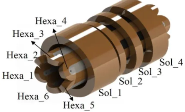
Therefore, in this paper, the characteristic analysis and protection circuit design are conducted toward the superconducting magnet for rare isotope science project (RISP) 28-GHz electron cyclotron resonance (ECR) ion source. To analyze the characteristics of superconducting magnet during quench, a numerical analysis code was developed for a solenoid coil by using MATLAB [1]. Also, the protection circuit is designed toward the hexapole superconducting magnet. In a design of the protection circuit, there is an assumption that the quench occurs in one of the hexapole magnet and does not propagate through the other magnets, since the assumption is a worst case. Fig. 1 shows the schematic drawing of superconducting magnet for RISP 28 GHz Ion source [2]. By using the developed simulation code, analytical results are compared with experimental results to verify the feasibility of simulation code. The analytical results are well agreed with the experimental results such as normal zone resistance, decaying current and temperature rising in the solenoid magnet. Also, the stored magnetic energy can be consumed from the series resistor of protection circuit. That is to say, current is well distributed through hexapole magnet and there is no overflowed current in all magnets. As the result, the developed characteristic analysis code can be used to estimate the characteristics of superconducting magnet
when the quench occurs. And the superconducting magnet is successfully protected using designed protection circuit.
2. QUENCH ANALYSIS OF SOLENOID MAGNET 2.1. Characteristic Analysis of Quench Propagation for Superconducting Magnet
To estimate the characteristics of superconducting magnet which is the biggest solenoid coil among the ECR ion source magnet, the numerical quench analysis code was developed. The superconducting wire is composed of copper and NbTi whose copper/NbTi ratio is 3.65. The superconducting wire is surrounded with an insulator, Formvar, and the epoxy is impregnated between superconducting layers.
Fig. 1. Schematic drawing of Superconducting Magnet for RISP 28-GHz ECR Ion Source.
Quench analysis and protection circuit design of a superconducting magnet system for RISP 28GHz ECR ion source
S. Songa, T. K. Koa, S. Choib, and M. C. Ahn*,c
a Yonsei University, Seoul, Korea
b Institute for Basic Science, Daejeon, Korea
c Kunsan National University, Gunsan, Korea
(Received 10 June 2016; revised or reviewed 26 June 2016; accepted 27 June 2016)
Abstract
This paper presents the developed quench analysis code and protection circuit design for a superconducting magnet system of 28GHz electron cyclotron resonance (ECR) ion source. The superconducting magnet is composed of a hexapole magnet and four solenoid magnets located outside of the hexapole one. All magnets are wound with NbTi composite wire and impregnated by epoxy.
By using the developed characteristic analysis code, the normal zone resistance, decaying current and temperature rising can be estimated during quench. Also, the stored magnetic energy is successfully consumed from the series resistor of the designed protection circuit. The analytical results are compared with the experimental results to verify the developed quench analysis code and protection circuit.
Keywords: ECR ion source, protection circuit, quench analysis, superconducting magnet
* Corresponding author: [email protected]
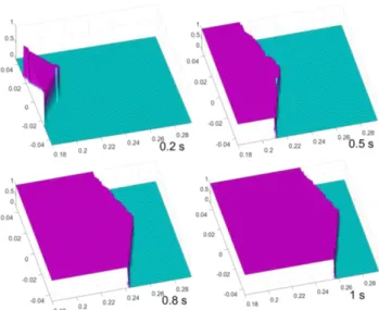
Fig. 2. Simulation results of the normal zone propagation from 0.2 s to 1 s.
The NZP velocity is calculated to estimate the normal zone volume fraction. We consider two dimensional NZP velocities; transverse (turn-to-turn) and longitudinal (along the conductor axis) NZP velocity. Those two velocities can be calculated as (1) and (2) [3-5]
) (
) ( ) ( ) (
~
~
~
0 t op
n n
l T T
T k T T
C U J
(1)
) (
) ( 2
1
~
~
T k
T U k
U
m i
i cd l
t
(2)
where Tt is transition temperature which is as the function of both magnetic field and current density of magnet, Top is operating temperature (4.2 K), T~ is average temperature from Top to Tt, J is current density, C0 is thermal capacity, ρn and kn are resistivity and thermal conductivity of matrix which are as a function of average temperature, δcd and δi are thickness of conductor and insulator, ki and km are thermal conductivity of insulator and matrix, respectively [1]. After acquiring the NZP velocity, the normal zone volume fraction (fr) should be considered to calculate the normal zone length and resistance. The fr is ratio of cross-sectional area to normal zone area of magnet in the resistive state. Fig. 2 shows the progress of normal zone propagation through the cross-sectional area of magnet from 0.2 s to 1 s. The normal zone resistance can be calculated using normal zone length. And the normal zone length is also calculated using fr as (3) and (4) [6, 7]
N a
fr
nz 1(1)
(3)
Rnz nAnz (4)
where a1 is inner diameter, α is ratio of outer diameter to inner diameter, N is total turns of magnet, ρn and A are resistivity and cross-sectional area of matrix. The temperature and current of the magnet can also be calculated as (5)
) ) ( ) (
( 2
~
~
~
t A I
T dt
T T d C
A op
m m cd
cd
(5)
where, Acd is area of conductor, Ccd is heat capacity of conductor, Iop is operating current, ρm and Am are resistivity and area of matrix metal [1, 7]. Fig. 3 shows some material properties used in the numerical analysis.
2.2. Comparison between Numerical and Experimental Results
The quench experiment was performed to acquire the data of current, temperature and internal voltage. Table I shows the specification of magnet which is used in the experiment. The resistance is calculated using voltage and current curves measured by data acquisition as (6).
(a)
(b)
Fig. 3. Material properties used in the numerical analysis;
(a) resistivity of copper and thermal conductivity of insulator, (b) Heat capacity and thermal conductivity of copper.
TABLEI
SPECIFICATIONS OF THE SOLENOID MAGNET.
Parameters Values
Number of turns 6400
Inductance 21.07 H
Inner radius (a1) 180 mm
Outer radius (a2) 294 mm
Height 92 mm
0 2 4 6 8
0 40 80 120 160 200
Experiment Simulation
Current (A)
Time (s)
0 3 6 9 12 15
Resistance
Resistance (ohm)
current
(a)
0 2 4 6 8
40 50 60 70 80
Temperature (K)
Time (s) (b)
Fig. 4. (a) Comparative results between experiment and simulation whose operating currents are 169 A. (b) Estimated final temperature of the magnet.
) (
) / ) ( ( ) ) (
( it
dt t di L t t V
Rnz (6)
where V(t) is the internal voltage, i(t) is the transporting current and L is the self-inductance of magnet. All data were obtained every 1 ms. Fig. 4 (a) shows the comparative results of experiment and simulation when operating current is 169 A. As shown in the results, current and resistance are well estimated. The estimated final temperature of the magnet is about 70 K.
3. PROTECTION CIRCUIT DESIGN OF A HEXAPOLE SUPERCONDUCTING MAGNET 3.1. Quench Analysis of Hexapole Superconducting Magnet
In order to calculate the current distribution among six hexapole magnets, the transient analysis is performed on electric circuit which is connected in series using developed characteristic analysis code. The current repartition of six hexapole magnets can be calculated as (7)
(7)
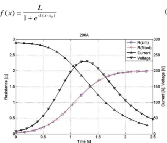
where L is the self-inductance, M is the mutual-inductance and R is series resistance which is essential to acquire current distribution among magnets. The inductance matrix is acquired by finite element method (FEM) tool, COMSOL Multiphysics. Table II shows inductance value (H) of hexapole magnet. And Table III shows specification of hexapole magnet. In order to calculate the current distribution among magnets, the series resistance should be calculated. Fig. 5 shows the experimental results of the first magnet whose operating current is 288 A during quench.
The same value of current is used in the simulation as the operating current of experiment. In the graph, voltage and current curves were acquired from experiment. And resistance curve is calculated using voltage and current curves. As shown in the results, resistance is increased exponentially for 1.3 s during internal voltage is increased and continue to rise up to 2 Ω for 0.7 s. And the resistance curve shows typical sigmoidal pattern. Therefore, in order to calculate the current distribution of hexapole magnets, the resistance curve is fitted using logistic function as (8)
) - (
- 0
+
=1 )
( k xx
e x L
f (8)
Fig. 5. Experimental results of 288 A during quench.
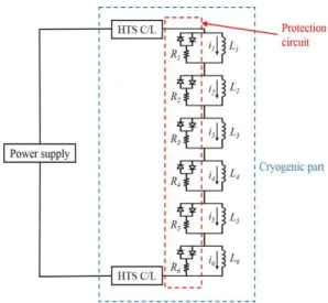
Fig. 6. Protection circuit of superconducting hexapole magnet.
TABLEII
INDUCTANCE OF HEXAPOLE MAGNET [H].
Hexa_1 Hexa_2 Hexa_2 Hexa_4 Hexa_5 Hexa_6 Hexa_1 1.1110 0.2109 -0.0583 0.0442 -0.0583 0.2112 Hexa_2 0.2109 1.1110 0.2109 -0.0583 0.0442 -0.0583 Hexa_3 -0.0583 0.2109 1.1110 0.2109 -0.0583 0.0442 Hexa_4 0.0442 -0.0583 0.2109 1.1110 0.2112 -0.0583 Hexa_5 -0.0583 0.0442 -0.0583 0.2109 1.1110 0.2112 Hexa_6 0.2112 -0.0583 0.0442 -0.0583 0.2112 1.1110
TABLEIII
SPECIFICATIONS OF HEXAPOLE MAGNET
Parameters Values
Number of turns 1367
Inner radius 108 mm
Depth 50 mm
Wire length 2.56 km / 1 unit
Conductor size 1.43ⅹ0.98 mm2
TABLEIV
SPECIFICATIONS OF DESIGNED RESISTOR
Parameters Values
Rod Diameter 2.5 mm
Length 2000 mm
Helix Diameter 30 mm
Turns 21
Length 100 mm
where L is the curve’s maximum value, k is the steepness of the curve and x0 is the x-value of the sigmoid’s midpoint.
The curve’s maximum value, the steepness of the curve and x-value of the sigmoid’s midpoint are 2.008, 3.79 and 1.069 respectively. Using the fitting curve, transient analysis was performed to get current data.
3.2. Current Distribution Analysis under Quench Condition Fig. 6 shows the protection circuit of hexapole magnet.
To protect the magnet, series resistor and back-to-back diode are used to dump the stored magnetic energy to resistor when quench occurs. Forward diode voltage drop of 2.5 V is considered to calculate the current distribution
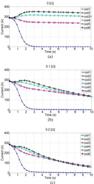
at each coil. Fig. 7 shows the simulation results of current repartition of hexapole magnet when series resistance is varied from 0 Ω to 0.2 Ω with 0.1 Ω increment. As shown in the graph (a), currents are not decayed when series resistance of 0 Ω is used except for coil 1 where the quench occurs. Also, currents overflow at coil 4 and 6 which can cause imbalance of electromagnetic force at the hexapole magnet. Therefore, series resistor is necessary to dump the stored magnetic energy to resistor. Graph (b) and (c) show the current distribution with the series resistance of 0.1 Ω and 0.2 Ω. As shown in the graph, current is decayed and balanced at each coil when the series resistor is used. Also currents are balanced at each coil after 5 s.
3.3. Design of series resistor
As shown in the simulation results of Fig. 7, current distribution is changed according to the value of resistance.
Therefore, it is required to calculate appropriate resistance.
The operating current is 288 A. And the same amplitude of series resistor is used in all hexapole magnets. Also, the current should not overflow in the hexapole magnets when the quench occurs. In this case the resistance of 0.2 Ω is appropriate.
In a design of a series resistor of 0.2 Ω, characteristics of stainless steel (SS316) is used. Because resistivity of SS316 is high at an extremely low temperature [8]. It is assumed that generating heat is only component to increase the temperature of resistor. Based on this assumption, length and cross-sectional area of resistor can be calculated as (9) and (10) [9, 10].
T ρC
R E
p m
= Δ
(9)
T RC
ρE S
p m
= Δ (10)
where Em is stored electromagnetic energy, R is resistance, ρ is resistivity and Cp is average heat capacity. Table IV shows the specifications of designed resistor. A rod with 2.5 mm diameter and 2 m length are wound in form of a cylindrical helix with 21 turns.
4. CONCLUSION
In this paper the characteristic analysis and protection circuit design is performed toward the ECR ion source magnet. To analyze the characteristics of the magnet, the simulation code was developed. As shown in the Fig. 4, the decaying current, normal zone resistance and hot-spot temperature were estimated iteratively using updated magnetic field and current density. And simulation results were compared with the experimental results to verify the feasibility of the developed code. The simulation results are well agreed with the experimental results.
Also, the protection circuit design of the hexapole magnet was performed based on the resistance curve which
(a)
(b)
(c)
Fig. 7. Current repartition of hexapole magnet with various series resistance.
is fitted using test results of internal voltage and current curves. As shown in the Fig. 7, current deviation of each magnet is decreased as series resistance is increased. From the simulation results, we selected the resistance of 0.2 Ω as a series resistor. And helix-type resistor is designed to protect hexapole magnet.
ACKNOWLEDGMENT
This work was supported by the Rare Isotope Science Project of Institute for Basic Science funded by Ministry of Science, ICT and Future Planning and National Research Foundation of Korea (2013M7A1A1075764).
REFERENCES
[1] S. Song, T. K. Ko, S. Choi, I. S. Hong, H. Kang and M. C. Ahn,
“Quench Analysis of a Superconducting Magnet for RISP 28 GHz ECR Ion Source,” IEEE Trans. Magn., vol. 25, no. 3, pp. xxx, 2015.
[2] H. Lee et al., “Electromagnetic characteristics of a superconducting magnet for the 28 GHz ECR ion source according to the series resistance of the protection circuit,” J. Kor. Phys. Soc. vol. 67, no. 8, pp. 1430-1434, 2015.
[3] G. Baccaglioni, M. Canali, L. Rossi and M. Sorbi, “Measurements of Quench Velocity in Adiabatic NbTi and NbSn Coils.
Comparison between Theory and Experiments in Small Model Coils and Large Magnets,” IEEE Trans. Magn., vol. 30, no. 4, pp.
2677-2680, 1994.
[4] C. H. Joshi and Y. Iwasa, “Prediction of current decay and terminal voltages in adiabatic superconducting magnets,” Cryogenics, vol.
29, pp. 157-167, 1989.
[5] C. H. Joshi, J. E. C. Williams and Y. Iwasa, “Quenching in Epoxy-Impregnated Superconducting Solenoids: Prediction and Verification,” IEEE Trans. Magn., MAG-23, no. 2, pp. 922-925, 1987.
[6] A. Ishiyama and Y. Iwasa, “Quench propagation velocities in an epoxy-impregnated Nb3Sn superconducting winding model,” IEEE Trans. Magn., vol. 24, no. 2, pp. 1194-1196, 1988.
[7] Y. Iwasa, Case Studies in Superconducting Magnets, Springer-Verlag, 2009.
[8] Y. M. Miura et al., “Development of Nb3Sn and NbTi CIC Conductors for Superconducting Poloidal Field Coils of JT-60,”
IEEE Trans. Magn., vol. 12, no. 1, pp. 611-614, 2002.
[9] C. A. Swenson et al., “Quench Protection Heater Design for Superconducting Solenoids,” IEEE Trans. Magn., vol. 32, no. 4, pp.
2659-2662, 1996.
[10] T. Rummel, O. Gaupp, G. Lochner and J. Sapper.,
“QuenchprotectionforthesuperconductingmagnetsystemofWendels tein7-X,” IEEE Trans. Appl. Superconduc., vol. 12, no. 1, pp.
1382-1385, 2002.