A Rule-based Urban Image Classification System for Time Series Landsat Data

1. Introduction

By understanding the surface changing mechanism, integrated management of land can be expected and the natural or artificial environment can be accurately verified. This study may be used as the basis for land planning and policy development by local governments

as well as to study the effect of natural and socio- economic factors on surface changes. Surface change caused by human behaviors can be verified by land registration or policy materials, but remote sensing has the advantage of periodic obtainment of past and present surface information and utilization of spectrum information (Park et al., 2001). In addition,

A Rule-based Urban Image Classification System for Time Series Landsat Data

Jin A Lee*, Sung Soon Lee**

and Kwang Hoon Chi*

*Dept. of Geoinformatic Engineering, University of Science & Technology

**Geoscience Information Department, Korea Institute of Geoscience and Mineral Resources

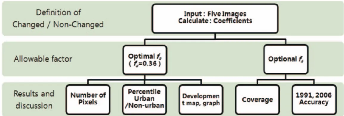
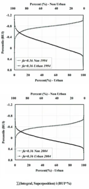
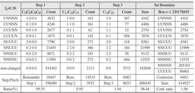
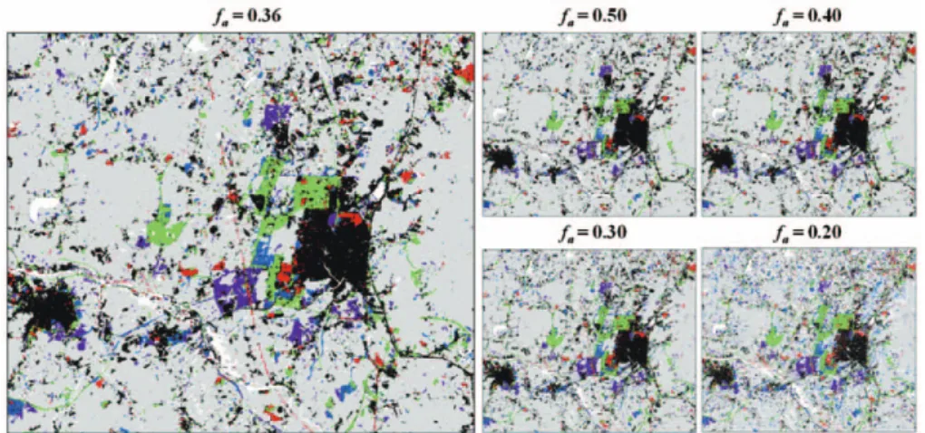
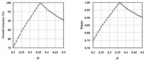
Abstract : This study presents a rule-based urban image classification method for time series analysis of changes in the vicinity of Asan-si and Cheonan-si in Chungcheongnam-do, using Landsat satellite images (1991-2006). The area has been highly developed through the relocation of industrial facilities, land development, construction of a high-speed railroad, and an extension of the subway. To determine the yearly changing pattern of the urban area, eleven classes were made depending on the trend of development. An algorithm was generalized for the rules to be applied as an unsupervised classification, without the need of training area. The analysis results show that the urban zone of the research area has increased by about 1.53 times, and each correlation graph confirmed the distribution of the Built Up Index (BUI) values for each class. To evaluate the rule-based classification, coverage and accuracy were assessed.

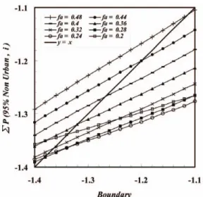
When Optimal allowable factor=0.36, the coverage of the rule was 98.4%, and for the test using ground data from 1991 to 2006, overall accuracy was 99.49%. It was confirmed that the method suggested to determine the maximum allowable factor correlates to the accuracy test results using ground data. Among the multiple images, available data was used as best as possible and classification accuracy could be improved since optimal classification to suit objectives was possible. The rule-based urban image classification method is expected to be applied to time series image analyses such as thematic mapping for urban development, urban development, and monitoring of environmental changes.

Key Words : Rule-based classification, Unsupervised-classification, Time Series, Chage Detection, Landsat

Received October 16, 2011; Revised November 10, 2011, Revised November 27, 2011; Accepted November 28, 2011.

†

Corresponding Author: Sung Soon Lee ([email protected])

vector machine (Knorn et al., 2009); a direct method is also used by object-oriented classification or screen digitizing of aerial images. No classification method can be said fundamentally superior to any other classification method. An algorithm suitable for proper results can be determined by priori knowledge in consideration of the problems and bio-physical characteristics of the study subject. Thus, different approaches must be explored considering the study objectives, and renewal of spatial information and its utilization are critical to securing scientific and economic values.

A number of studies are being conducted to overcome the limitations of classification using only single image spectrum information and data collected from each sensor (Yeom et al., 2011). Furthermore, there are other studies being conducted in order to improve classification accuracy for a study area using images of multiple periods in which there is little change. In addition, time series analysis can be done using the subtraction method (Krishnaswamy et al., 2009) to detect changes in images from multiple periods, as well as by using the post classification comparison method (Alphan et al., 2009; Yuan et al., 2005). Geo-spatial data can be integrated by a number of approaches such as hierarchical application of integrated data, introduction of an artificial neural network, the statistical approach, and the use of fuzzy functions. Macro decision-making is

also provides a performance compatible to that of other classification methods such as a decision tree (Liu et al., 2000). Accordingly, if rule-based classification is used along with remote sensing to perform automated image classification, multi-data processing and classification can be effectively conducted to achieve the goals(Lawrence and Wright, 2001; Rogan et al., 2003; Wright and Gallant, 2007).

Thus, along with generalization of the process, its justification must be proven through a comparison with other techniques and its reliability needs to be tested (Coenen and Leng, 2007).

This study is to perform and test a rule-based urban image classification system using satellite images of multi-periods of the Asan-Cheonan region (Fig. 1).

First, continuity data of the satellite images was

defined not by a single property, but by multiple

properties, and a rule-based image classification of

the changed/non-changed areas depending on the

sequential development trend was suggested. Second,

the statistical/mathematical method for rule-based

classification was generalized so as to perform quality

unsupervised classification. Third, coverage was

checked to evaluate the classification rules, and

classification accuracy was checked by sample data

obtained from ground data to evaluate the

classification results. Furthermore, the rule suitability

was checked by the correlation between the equation

for the optimal allowable factor and classification

accuracy. By suggesting an optimized and reasonable method to determine and integrate development changes using images of multiple periods, the suggested method was proven to be an excellent way to effectively detect land development changes.

2. Study area and rule-based classification

1) Study area and used material

The study area is the Asan-Cheonan-si region in Chungcheongnam-do (about 373.4 km

). The population increased a lot because of the expansion of

road networks and infra-structure in the 2000s. In April 2004, Cheonan-Asan station, a high-speed railroad station, was constructed, and in January 2005, construction for a subway between Cheonan and Seoul was completed. The reason why the population of Cheonan has exploded appears to be because of the collateral benefits to the area from the dispersion policy of the greater Seoul region: both people and industries have moved to the northern part of Cheonan.

To perform the time series change detection, Landsat images of (1) 1991.08.28TM, (2) 1994.08.20TM, (3) 2001.09.16ETM+, (4) 2004.08.31TM, and (5) 2006.09.22TM (Fig. 2) were used. Using unified Fig. 1. Flowchart for the overall data processing of the study.

Fig. 2 . Landsat TM ETM+ satellite images (RGB) of the study area. (a) 1991.08.28TM (b) 1994.08.20TM (c) 2001.09.16ETM+ (4) 2004.08.31TM and (5) 2006.09.22TM (f) Administrative district.

(a) (b)

seasonal images, geometric modification of images from 2006 was conducted for the digital map with the scale of 1:25,000 based on the ground control point, other images were geometrically modified, and the image to image method was also used. Raster data of 30m×30m obtained were converted to ASCII code values to be used in this study.

2) Built-up index (BUI)

The urban area has a relatively greater Built-up Index (BUI), which uses the difference between NDVI and NDBI, whereas the rural area has a smaller BUI (Zha et al., 2003). The urban area (U)

includes commercial land, public land, residential area, and vacant land, whereas the non-urban area (N) includes forests, fields, farmlands, and parks. The river/stream needs to be excluded using the stream space information of the area because its BUI is very irregular and has a negative effect.

NDBI = (1)

NDVI = (2)

BUI = NDBI _ NDVI (3) NDBI: normalized difference built-up index

NDVI: normalized difference vegetation index MidIR

_ RED

MidIR

+ RED

MidIR

_ NIR

MidIR

+ NIR

Fig. 2 . continued

(e)

(c) (d)

(f)

BUI: built-up index (Zha et al., 2003)

In case of continuous data having a quantitative value, binary classification is possible, but actual satellite images cannot be optimally classified using the conditions of a single property (Li et al., 2011;

Wang and Feng, 2011). In analyzing the BUI distribution of two different periods, the changed area has BUI values that have increased or decreased.

Using the relation, changes in land coverage can be verified. When conducting a regression analysis on the BUI distribution of two images (Table 1), as the time gap is increases, the coefficient of determination (R

) decreases. This is because the larger the changed area, the smaller the correlation.

3) Rule-based classification system

Rule-based classification is a method to classify using a set of “If…Then…” rules. The quality of the rules can be evaluated using assessment criteria such as coverage or accuracy (Liu et al., 2000). As a principle for the rule-based classification system, mutually exclusive rules and exhaustive rules need to be applied. If a set of rules has both mutual exclusivity and exhaustiveness, each individual item can be applied exactly to one rule. If the set of rules is not exhaustive, a default rule needs to be added so

that it can be applied to residual cases. Generally, these cases are all remaining items that cannot be applied to the existing rules. When automatically processing useful information from large data, data relations need to be considered to process complicated data (Coenen and Leng, 2007).

There are direct methods and indirect methods such as decision making trees or neural networks to deduce classification rules. This study required logical determination of direct rules that create relative equations by the BUI distribution characteristics in the unban/non-urban areas and that is suitable for final objectives depending on the sequential development trend in time series images (Wright and Gallant, 2007).

First, generalized equations were allowed for automatic calculation and their application to other research areas or other time periods was essential.

They were determined by the BUI distribution of five time period images. The consistent rule of the BUI was verified to determine the characteristics of a pixel by mutual reaction. Second, class can be defined by the sequential development trend using the definition of changed/non-changed. Ten classes of changed (Built up: NUUUU-NNUUU-NNNUU-NNNNU, Greening: UNNNN-UUNNN-UUUNN-UUUUN) Table 1. Correlation statistics of the BUI for each image

Image Year BUI(All) BUI (Percentile)

i j i j R

mij tij R

1 2 1991 1994 0.597789 1.026822 -0.007742 0.998423

2 3 1994 2001 0.393017 0.990679 0.466649 0.982119

3 4 2001 2004 0.569720 0.810236 -0.169637 0.996668

4 5 2004 2006 0.599386 1.030236 -0.081143 0.997448

1 3 1991 2001 0.314816 1.016209 0.458430 0.978562

2 4 1994 2004 0.409488 0.804137 0.209257 0.982391

3 5 2001 2006 0.515650 0.836668 -0.255760 0.998733

1 4 1991 2004 0.326723 0.825649 0.203001 0.980708

2 5 1994 2006 0.323836 0.826314 0.133266 0.974837

1 5 1991 2006 0.251504 0.848159 0.126701 0.972570

Image Year BUI(All) BUI (Percentile)

i j i j R

m

t

R

and non-changed(NNNNN, UUUUU) and a confusion class by a default rule were set. Third, if several ground objects were included in one pixel, image data cannot be representative, and thus, if there was a small error, it could be assigned to a proper class using an additional rule (Fig. 3).

4) Definition of changed/non-changed In processing a plurality of continuous data, average and deviation may be representative, but they are sensitive to each variable. Here, observed values such as percentile are needed for evaluation.

Similarity criteria were suggested using percentile (99,95,90,75,50,25,10,5,1%), excluding the maximum and minimum values. They show a strong first-order linear relation (Table 1). This is an efficient method to determine the differences in images from different periods. The difference in the characteristics of each band for TM and ETM+ images was also minimized using the BUI and coefficient setting by the correlation. Photographing conditions and data characteristics were modified to be reflected in the

calculation.

To define the dissimilarity criteria for data objects having multiple properties, the distance matrix (D

) was defined and the boundary was set to determine the non-changed area.

y

= m

·x

+ t

(4)

D

= (5)

l

= P

_ P

(6)

L

= (7)

where P

, P

= BUI(built-up index) value in i, j images m

= linear regression slope

t

= linear regression intercept D

= distance between y

and (P

, P

) l

, l

= BUI length (i) (j)

L

= BUI length (i, j)

Classification for each step is conducted using the characteristic value matrix (8, 9, and 10) for the classification of changed (built-up, greening)/non- changed.

l

·l

l

+ l

m

·P

+ t

_ P

m

+ 1

Fig. 3. Rule-based classification system.

If D

< _ f

L

Then C

= 2 (changed : built-up) (8) If D

> f

L

Then C

= 1 (changed : greening) (9) If _ f

L

D

f

L

Then C

= 0 (non-changed) (10) where f

= allowable factor, threshold value

C

= the characteristic value matrix

For non-changed (NNNNN,UUUUU), the 95%

percentile value of the non-urban area was calculated by setting a random boundary value, and this process was repeated to calculate a limited boundary value.

Depending on the boundary value, five images from the 95% percentile of the non-urban area are combined. Here, if the value was same, the limited boundary was calculated by convergence, and each (Boundarylim) could be calculated for each allowable factor (f

)(Fig. 4).

In non-changed,

If P

≥ Boundary Then UUUUU (11)

If P

> Boundary Then NNNNN (12)

In Non Urban Classes,

(13) (95%, Percentile)

Boundary

5) Definition of optimal allowable factor In the process, an allowable factor (f

) can be inputted by a user depending on the range of the objective (0.25-0.5), or if there is no input, the optimal allowable factor is statistically calculated to perform classification. Rule-based classification produces a result different from that by binary classification. The distribution of the BUI, continuous data, has separation distance in the non-urban/urban sets. Separation distance is calculated depending on the allowable factor, and the optimal separation value needs to be deduced. Here, when the overlapping area is smallest, separation can be said to be proper.

The BUI percentile values of the non-urban/urban sets for each of the five images, excluding confusion class, were calculated with a 0.1% increment (Fig. 5).

The superposition area (overlapping area) was calculated for each of the five graphs and summed.

Here, the area summation was graphed and smallest when f

= 0.36.

3. Rule-based image classification result

1) Calculation of the rule-based urban image classification

Once B3, B4, B5, stream information, and administrative district information of an image were entered to the classification system in ASCII code, correlation equations among the images were calculated based on the given data. Changed (built- up, greening)/non-changed classification was conducted using the characteristic value matrix.

Output data is in the form of a DBF file, including statistics for each image, a classification summary (Table 2), and the class classification results; output data can be converted to raster data.

Step 1 covers cases satisfying all rules of the first

S

S

S

Fig. 4. Process to calculate limited boundary.

Fig. 5. BUI distribution for non-urban/urban sets. Summation of the overlapping area for each allowable factor.

period and Steps 2 and 3 cover non-classified cases respectively satisfying the rules of the second and third periods to be re-assigned to a class. Others were assigned to the confusion class (default class). Step 1 shows about 95.55% of high coverage satisfying all rules and being classified. Furthermore, reassigned

areas in Steps 2 and 3 are only about 2.89%. There are not many areas classified as the confusion class, which were mainly distributed at the boundaries of the narrow road vicinity, stream vicinity, or complex regions. The classification results show that the urban area increased by about 1.53 times from 1991 to Table 2. Number of pixels classified to each class and by each step

f

=0.36 Step 1 Step 2 Step 3 Set Boundary

C

C

C

C

Count C

C

C

Count C

C

Count Sum Bou.=-1.320178845

UNNNN 1 0 0 0 3632 1 0 0 163 1 0 367 4162 UNNNN 4162

UUNNN 0 1 0 0 4248 1 1 0 161 1 1 77 4486 UUNNN 4486

UUUNN 0 0 1 0 2677 0 1 1 62 1 1 15 2754 UUUNN 2754

UUUUN 0 0 0 1 1875 0 0 1 145 0 1 958 2978 UUUUN 2978

NUUUU 2 0 0 0 7790 2 0 0 273 2 0 318 8381 NUUUU 8381

NNUUU 0 2 0 0 21455 2 2 0 360 2 2 184 21999 NNUUU 21999

NNNUU 0 0 2 0 8871 0 2 2 183 2 2 58 9112 NNNUU 9112

NNNNU 0 0 0 2 11569 0 0 2 272 0 2 684 12525 NNNNU 12525

non-changed 0 0 0 0 334363 0 0 0 2313 0 0 5372 342048 NNNNN 285183 UUUUU 56865 Step,Pixels Remainder 18447 Rem. 14515 Rem. 6482 Confusion 6482 Step 1 396480 Step 2 3932 Step 3 8033 408445 Sum 414927

Ratio(%) 95.55 0.95 1.94 98.44 Conf. ratio 1.56

f

=0.36 Step 1 Step 2 Step 3 Set Boundary

C

C

C

C

Count C

C

C

Count C

C

Count Sum Bou.=-1.320178845

Table 3. The percentile value of the non-urban classes (the limited boundary)

Image 1991 1994 2001 2004 2006 S P (n%)

NUUUU UNNNN UNNNN UNNNN UNNNN

Classes NNUUU NNUUU UUNNN UUNNN UUNNN Bou.=

Non (f

=0.36) NNNUU NNNUU NNNUU UUUNN UUUNN -1.320178845

-urban NNNNU NNNNU NNNNU NNNNU UUUUN

NNNNN NNNNN NNNNN NNNNN NNNNN

Pixels 337200 332981 315468 309110 299563

100 0.533189 0.169935 0.731858 0.410957 0.350602 2.196540334 99 -0.280380 -0.344406 0.271652 -0.023099 -0.062607 -0.438839336 95 -0.459891 -0.510086 0.048423 -0.169393 -0.229231 -1.320178845 Non 90 -0.538934 -0.595011 -0.053044 -0.244253 -0.312432 -1.743675521 -urban Per 75 -0.639623 -0.706122 -0.218891 -0.345388 -0.443326 -2.353351353 -centile (%) 50 -0.729460 -0.787583 -0.348969 -0.418655 -0.539683 -2.824349214 25 -0.831413 -0.863473 -0.425059 -0.482773 -0.609260 -3.211977287 10 -0.908561 -0.930722 -0.478467 -0.564189 -0.663636 -3.545575879 5 -0.934072 -0.958088 -0.507476 -0.605063 -0.692928 -3.697628179 1 -0.969872 -0.996947 -0.558569 -0.656710 -0.745299 -3.927397279 0 -1.136585 -1.161513 -0.789249 -0.800160 -1.012821 -4.900327416

Image 1991 1994 2001 2004 2006 S P (n%)

Bou.=

-1.320178845

-1.320178845

2006. The percentile values of the non-urban area (Table 3) was calculated by setting a limited boundary value (-1.320178845).

2) Visualization of the rule-based urban image classification

Gradual development was done in the vicinity of Cheonan-Asan station, which was constructed for a high-speed railroad. The development included Cheonan City Hall relocation, residential district development, and industrial facility relocation. The area was classified by Step 1 as UUUUU, NUUUU, NNUUU, NNNUU, NNNNU, and NNNNN. If the correlation of 1-2, 2-3, 3-4, and 4-5 periods was described for each class, how the classification is performed could be checked. The changed (built-up) area shows for each period of NUUUU (2000), NNUUU (0200), NNNUU (0020), and NNNNU (0002), and the area is on the top left side of the correlation graph. The non-changed area is within the similarity range, but UUUUU shows a high BUI for all five periods, whereas NNNNN shows a low BUI

(Fig. 6).

3) Classification result for each allowable factor

If the six classes are described in colors, a thematic map of the development trend can be created (Fig. 7).

Class classification shows the development trend and areas, and large and small scale changes can be retrieved. In addition, future development areas can be predicted.

4. Evaluation of the classification method

1) Evaluation of coverage of the rule-based classification

The quality of classification rules can be evaluated

based on measurement tools such as their coverage

and accuracy. If a set of rules has both mutual

exclusiveness and exhaustiveness, each individual

Fig. 6. Classification result of point areas.

item is applied to one rule. If the set is not exhaustive, a default rule needs to be added to cover the remaining cases (Liu et al., 2000). While exploring mega-size data for useful information, data relations should be considered to process complicated data. In the data exploration, over 80% is classified in Step 1, and thus, the rules appear to be appropriate (Fig. 8).

As the allowable factor increases, the larger area is considered non-change and coverage increases.

2) Classification accuracy of the rule-based classification

To test the suitability of an image classification

method, a field study, high resolution image, or digital map is used, but timeliness, information availability, and economic feasibility must be considered. Thus, if the unsupervised classification method secures a certain level of quality of classification, it can be concluded to have utility (Yuan et al., 2005). The suggested rule-based urban image classification method is distinct because it is not used to classify a single image, but to integrate and classify multiple images of different periods. Five images were used in this study and three or more images may be used. It is desirable to use as many images as possible because more reference data means more rules.

Ground data from 1991.08.28 and 2006.09.22 in a digital map with a scale of 1:25,000 were used to test land coverage. The digital map was partially modified in some areas to be applied. To prevent an analyzer’s subjective perspective in retrieving sample data, a principle was set to depend on the vector data of the digital map. However, the pixel size of the satellite image is 30 m×30 m, and thus, areas with vague boundaries or small areas were excluded from test samples.

To test accuracy, non-urban, urban, and confusion areas in 1991 and 2006 were classified and both Fig. 7. Comparison of the rule-based image classifications of the Asan-Cheonan area for each allowable factor

Fig. 8. Coverage for each allowable factor.

periods were calculated for classification accuracy (Table 4, Fig. 9). Classification results from the suggested rule-based classification showed high producer accuracy and user accuracy, and when f

= 0.36, Kappa = 0.9948, proving the reliability of the classification results. Classification standards vary depending on the allowable factor, and accuracy assessment varies accordingly.

3) Optimal allowable factor and accuracy assessment

The objectives of this study are to perform unsupervised classification of images without the need for a training area, to suggest a logical method suitable for time series image analysis, and to prove

the method’s utility. The information from five images was integrated to be classified suitable for the purpose according to the BUI characteristics and distribution of each image, and thus, classification accuracy has been expected to improve.

Classification was performed by mutually exclusive and exhaustive rules and the non-urban/urban classification results of different periods referred to each other. Given that the accuracy assessment of the classification results from 1991 and 2006 proved the reliability of the rule-based classification, quality classification of different periods can be expected.

Even without test material using ground data, it is desirable to secure a certain degree of classification Fig. 9. Accuracy assessment of the allowable factor. Overall accuracy and Kappa.

Table 4. Accuracy assessment for allowable factor

Producer’s Accuracy User’s Accuracy Overall

Kappa f

Accuracy (%)

N-N N-U U-N U-U N-N N-U U-N U-U

0.48 99.44 67.48 37.14 85.75 92.24 94.08 78.00 86.70 91.39 0.9126 0.44 99.35 76.46 51.43 91.38 94.68 95.31 82.44 89.60 93.73 0.9364 0.40 99.60 86.77 70.00 95.69 97.05 97.41 91.88 93.62 96.44 0.9639 0.36 99.64 99.03 99.52 99.12 99.96 98.19 97.66 99.45 99.49 0.9948 0.32 95.70 91.87 89.52 89.72 99.33 83.37 66.67 95.31 94.17 0.9408 0.28 91.08 87.14 78.57 79.23 98.89 70.19 43.42 94.09 88.50 0.8834 0.24 85.44 82.89 68.57 68.51 98.74 58.38 28.97 94.51 82.18 0.8196 0.20 78.32 80.34 60.00 58.67 99.07 49.89 19.30 97.07 75.22 0.7494

Producer’s Accuracy User’s Accuracy Overall

f

Accuracy Kappa

N-N N-U U-N U-U N-N N-U U-N U-U (%)

accuracy. It is suggested to regard as the optimal coefficient, which can minimize the overlapping area of the non-urban/urban BUI distributions. The utility of this method needs to be reviewed. Using the test material from 1991 and 2006, the overlapping area and classification accuracy for each coefficient have a significant correlation. The allowable factor with a small overlapping area actually showed high accuracy (Fig. 10).

5. Conclusion

To perform a time series analysis on the Asan- Cheonan vicinity to see ground changes between 1991 and 2006, a rule-based urban image classification method was applied and its results were tested.

The different BUI characteristics of urban and non- urban areas may be reflected, but it is continuous data that cannot be optimally classified as a single property. Thus, to process multiple continuous data, a similarity standard was suggested for the percentile of multiple period combinations and a dissimilarity scale

was defined by calculating each distance matrix.

Changed (built-up, greening)/non-changed classes were classified and a rule was added to reclassify data if there was a small error. It is critical to set rules to be mutually exclusive and exhaustive.

The Asan-Cheonan area classification results were confirmed for each class. For the optimal allowable factor of f

= 0.36, Step 1 showed 95.55% coverage.

For each period, the urban area increased, and between 1991 and 2006, it increased by about 1.53 times. Using ground material from 1991 and 2006, Kappa was 0.9948, proving the reliability of the classification results. The allowable factor could be set by a user to change the range to determine the non-change area. Or the non-urban/urban BUI distribution overlapping area was calculated and when it as small as possible, the allowable factor was considered optimal. Here, the optimal allowable factor was f

= 0.36, and it shows greatest overall accuracy in the actual assessment. As the overlapping area increases, accuracy increases, and thus, this proves that the method to calculate the optimal allowable factor is correct.

The objective of this study is to generalize equations and rule applications for the entire process of creating the rule-based classification method so that quality unsupervised classification can be performed by inputting ASCII values of images from other areas for the same season, irrespective of users.

Classification results of multiple periods were able to refer to each other to improve classification accuracy and the test results show such a quality classification result. It also has utility since reliable classification results suitable for the purpose were obtained by processing data from a large region. Further study on universality is necessary for satellite images obtained from other sensors. The results of this study can be used for new city development planning or local government policy assessment, and can be used in Fig. 10. Correlation between overlapping area of the

nonurban/urban BUI distribution and overall accuracy.

References

Alphan, H., H. Doygun, and Y.I. Unlukaplan, 2009.

Post-classification comparison of land cover using multitemporal Landsat and ASTER imagery: the case of Kahramanmaras, Turkey, Environmental Monitoring and Assessment, 151(1-4):327-336.

Coenen, F. and P. Leng, 2007. The effect of threshold values on association rule based classification accuracy, Data & Knowledge Engineering, 60(2): 345-360.

Jeneratte, G.D. and D. Potere, 2010.Global analysis and simulation of land-use change associated with urbanization, Landscape Ecology, 25(5):

657-670.

Knorn, J., A. Rabe, V.C. Radeloff, T. Kuemmerle, J.

Kozak, and P. Hostert, 2009. Land cover mapping of large areas using chain classification of neighboring Landsat satellite images, Remote Sensing of Environment, 113(5): 957-964.

Krishnaswamy, J., M.C. Kiran, and K.N. Ganeshaiah, 2004. Tree model based eco-climatic vegetation classification and fuzzy mapping in diverse tropical deciduous ecosystems using multi-season NDVI, International

engineering and Remote Sensing, 67(10):

1137-1142.

Lee, S.W. and N.W. Park, 2011. Application of Bayesian probability rule to the combination of spectral and temporal contextual information in land-cover classification, Korean Journal of Remote Sensing, 27(4): 435-444.

Li, W, Z. Ouyang, and W. Zhou, 2011. Effects of spatial resolution of remotely sensed data on estimating urban impervious surfaces, Journal of Environmental Sciences, 23(8):

1375-1383.

Liu, B., Y. Ma, and C.K. Wong, 2000. Improving an association rule based classifier, In Proceedings of PKDD’2000, pp. 504-509.

Liu, H. and Q. Zhou, 2004. Accuracy analysis of remote sensing change detection by rule- based rationality evaluation with post- classification comparison, International Journal of Remote Sensing, 25(5): 1037- 1050.

Park, G.A, I.K. Jung, M.S. Lee, H.J. Shin, J.Y. Park, and S.J. Kim, 2008. Analysis of Land Use Change Impact on Storm Runoff in Anseongcheon Watershed, Korean Journal of Remote Sensing, 24(1): 35-43.

Park, S.M, J.H. Im, and H.S. Sakong, 2001. Land

Cover Classification of a wide Area through

Multi-Scene Landsat Processing, Korean

Journal of Remote Sensing, 17(3): 189-197.

Rogan, J., J. Miller, D. Stow, J. Franklin, L. Levien, and C. Fischer, 2003. Land-cover change monitoring with classification trees using Landsat TM and ancillary data, Photogrammetric Engineering and Remote Sensing, 69(7): 793- 804.

Wang, Y.C. and C.C. Feng, 2011. Patterns and trends in land-use land-cover change research explored using self-organizing map, International Journal of Remote Sensing, 32(13): 3765-3790.

Wright, C., and A. Gallant, 2007. Improved wetland remote sensing in Yellowstone National Park using classification trees to combine TM imagery and ancillary environmental data, Remote Sensing of Environment, 107(4): 582- 605.

Yeom, J., J. Lee, D. Kim, and Y. Kim, 2011.

Hierarchical Land cover classification using IKONOS and AIRSAR images, Korean Journal of Remote Sensing, 27(4): 435-444.

Yuan, F., K.E. Sawaya, B.C. Loeffelholz, and M.E.

Bauer, 2005. Land cover classification and change analysis of the Twin Cities (Minnesota) Metropolitan Area by multitemporal Landsat remote sensing, Remote Sensing of Environment, 98(2-3): 317-328.

Zha, Y., J. Gao, and S. Ni, 2003. Use of normalized

difference built-up index in automatically

mapping urban areas from TM imagery,

International Journal of Remote Sensing,

24(3): 583-594.