AN ANALYSIS OF CHANGES IN SURFACE TEMPERATURE IN RELATION TO VARIATIONS OF INDUSTRIAL ACTIVITIES
Jin A, Lee Sung Soon, Lee Kwang Hoon, Chi
Dep.Geoinformatic Engineering, University of Science & Technology, [email protected]
Geoscience Information Department, Korea Institute of Geoscience and Mineral Resources, [email protected] Korea-Japan Cooperation Foundation for Industry and Technology, [email protected]
ABSTRACT ... Surface temperature measurement made through remote sensing is widely used in the areas of weather, environment, forest and water resources. Diverse studies that extract surface temperatures and interpret causal relations with related factors are currently being conducted. This paper attempted to analyze the trends of changes in surface temperature for industries in up-phases and those in recessions. To this end, the surface temperatures in industrial complexes in Daegu during the period of 1997~2003 were calculated. During this period, Korea experienced the IMF economic crisis, and the industrial complexes in Daegu were greatly affected by the industrial recession.
Surface temperatures were calculated using the Landsat B6. Surface temperature distribution in relation to the arrangements of industrial complexes and factories was identified. The results showed that the surface temperatures in industrial complexes were higher than those located downtown or in agricultural areas, and their yearly changes were relatively larger. Forty-five businesses in the ‘Daegu Dyeing Industrial Center’ were sampled in order to analyze surface temperature dT by industry type. Of the samples, 30 businesses showed significant surface temperature decreases in 1997~1999. This result was analyzed along with statistical values of various industrial complexes and the trends of industrial activities to prove significant correlations. Later, site monitoring and additional studies on diverse industrial categories will be conducted. This study may be utilized as basic data for analyses of the urban industrial economy.
KEY WORDS: Thermal band, Surface Temperature, Landsat, Time series, GDP
1. INTRODUCTION
As a result of the development of remote sensing, more information can now be obtained and many studies are being conducted using this new data. This study is intended to compare various images obtained during the period of 1994~2003 in order to evaluate surface temperatures in manufacturing areas that have changed due to economic conditions.
Although spatial distribution of surface temperatures can periodically be obtained, it has been difficult to consider seasonal changes, the height of the sun on the dates of photographing and differences in atmospheric temperatures and humidity. Therefore, studies conducted to date can be said to have interpreted and compared phenomena in short periods.
The possibility to estimate temperature distributions in relation to the state of the shell on the earth’s surface through analyses of correlations between the vegetation index and surface temperatures has been evaluated (Griend, 1993). Studies by Lambin (1996) and Griend (1993) have shown that radiated surface temperatures are closely related to the surface water content and vegetation indexes. Lee (2004) analyzed urban surface temperatures, land shells and vegetation indexes along with topographical factors. He elucidated spatial distribution characteristics and suggested using the characteristics as basic data in establishing city plans. In addition to studies relating to cities, mapping of coal fires has been conducted using thermal images (Prakash, 1999;
Chatterjee, 2006). Lagios (2007) reported that there are differences ranging from approximately 0 to 2 ℃ between surface temperatures obtained through site observations and those obtained through thermal images.
As such, diverse studies are being conducted that do not only extract surface temperatures from remote sensing data but also interpret causal relationships with related factors as well as using them.
Daegu is a heavily industrialized manufacturing city that has undergone drastic changes over the years and therefore was selected for our study region. Surface temperatures in the region were calculated using the thermal bands of Landsat TM5 and ETM7. Temperature decreases/increases in large factories with the same type of operations were obtained, and methods to select representative values were identified. Correlations between the values obtained and the manufacturing industry’s GDP were derived.
2. SCOPE OF THE STUDY 2.1 Study period and region
Korea requested a relief loan to IMF in November 1997. Conditions of many businesses had deteriorated and many people had lost their jobs. The GDP growth rate in 1998 dropped to -6.9%, but businesses have since recovered, and the growth rate was recorded as 7% in 2002 and 3.1% in 2003. In Daegu, which is an industrial city, the unemployment ratio in May 1997 was 3.5%, but
this was recorded as 8.0% in 1998 and 7.6% in 1999.
This time period has thus shown clear industrial recessions and recoveries (KOSIS, 2009).
The GDP in the manufacturing industry has been generally growing but showed downward trends after the second quarter in 1997 (Figure 1). The GDP for each quarter in 1998 was lower by at least 5 trillion won compared to the previous increasing trends. (The values for 1999 and earlier years were prepared based on prices in 2000 and were re-calculated by applying growth rates.)
Figure 1. GDP and GNI by type of economic activity (at chained 2005 prices, SA).
Korea has administrative districts divided into seven metropolitan cities, including Seoul, Busan, Daegu, Incheon, Gwangju, Daejon and Ulsan and nine provinces.
Among them, Daegu has an area of 884.15km2 where 2,512,604 people (5.4% of the population of Korea) lived as of December 31, 2008. Daegu has led the industrial economy of Korea since the 1970s. Sizes of textile, machine and equipment and car component industries are large, and approximately 97,000 people engage in manufacturing. It is a representative basin-type city showing the highest temperatures in the summer.
Table 1. The number of all businesses in three industrial complexes and the number of business that closed or
leased facilities to others.
For this study, information on the industrial complexes, including tenant businesses, operating businesses, production amount and the number of personnel, were surveyed by type of business. Information on businesses that were closed or facilities that were leased to other companies were included (Table 1). Based on the results, the number of businesses that closed or leased facilities to others were shown to have increased remarkably during the IMF period.
2.2 Calculation of DATA and surface temperatures Images from April and May of band 6 of Landsat TM5 and ETM7 were used (Table 2). The images were obtained on days that followed a 3-day period of no cloud cover and no rain.
Table 2. Image list and temperatures and the height of the sun at the times of image capture.
Band 6 of Landsat was used to establish the surface temperature map of Daegu and elucidate surface temperatures by factory and by complex. The images were geometrically corrected using a 1:5000 numerical topographical map. The GCP error was controlled to be less than 0.2. Spectral radiance values were calculated for each DN of Landsat band 6, and surface temperatures were extracted using the coefficients of the NASA method (Chander, 2003 ; NASA, 1998).
3. PROPOSAL OF A METHOD OF TIME SERIES ANALYSES
Xian (2006) divided images taken from the study region at two different time points based on the scope of impervious surface area (ISA) and obtained the average surface temperature of each of them. The surface temperatures with ISA < 10% were calculated by the formula: ΔTb = T-T(ISA<10%) based on the average surface temperature T. In this study, this method was applied for standardization of time series analyses.
Places that are free of external changes and not affected by vegetation or moisture should be selected.
Y/ M/ D Landsat Path Low
Atm.
Temp (℃)
Sun Azimuth
Sun Elv.
19940509 5 TM 114 35 20.4 118 58 19950512 5 TM 114 35 15.2 113 56 19960403 5 TM 115 35 5.3 126 46 19970517 5 TM 114 35 21.4 118 61 19980520 5 TM 114 35 22.8 120 63 19990507 5 TM 114 35 22.3 124 60 20000508 7 ETM 115 35 20.4 128.2 62.8 20010418 7 ETM 114 35 19.4 134.3 57.1 20020523 7 ETM 114 35 23 121.5 64.6 20030510 7 ETM 114 35 16.3 126.4 62.5
ALL Closed
or Lease ALL Closed
or Lease ALL Closed or Lease
1994.5 484 16 112 1
1995.5 1169 336 112 0
1996.5 1093 176 113 8
1997.5 1134 74 254 42 113 12
1998.5 1183 206 259 54 113 14
1999.5 1198 256 265 49 113 10
2000.5 1232 171 281 24 110 6
2001.5 1259 211 283 23 113 8
2002.5 1318 254 299 14 117 8
2003.5 1655 303 322 19 117 8
Seong-Seo Dal-Seong Dyeing Industrial
Y.M
Therefore, the surface temperatures of large playgrounds of 50 schools located in downtown Daegu were surveyed.
Cluster analyses were conducted with a total of 255 observed values, and the quartile values and the average value of the final 104 observed values were obtained.
The observed values of each time point satisfied normality, and their standard deviations had values ranging from 0.59 to 0.84. The average values of individual quartile values and observed values are shown in Figure 2.
Figure 2. The quartile values and average values of 104 observed values of individual images.
n Tp,y =
∑
tplayground,y(1)
where Tp,y = the observed value(˚C) that will become the reference value for the values of the playground in the year
y = Year, 1994~2003
n = the number of observed values = 104 t = observed values of the selected playground
y p y y
n
T T
T
,= −
, (2)where Tn,y= Nomalized surface temperature values of individual pixels (˚C)
Ty = temperatures of individual pixels calculated in the thermal band (˚C)
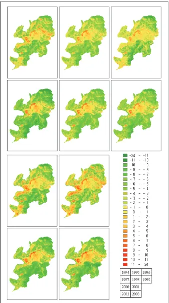
The average values for 104 points in the playgrounds were calculated by formula (1). The values were different for different dates of photographing. Using formula (2), temperature distribution diagrams were made for the entire Daegu region, using Tn,y values (Figure 3).
Downtown areas show values close to 0, mountain areas show negative values and the industrial complexes located on the northwest side are in red.
Figure 3. Temperature distribution diagrams for Daegu, Tn,y (℃).
The ratios of the areas with Tn,y values smaller than 0 were calculated (Table 3). Sindang-ri and Gyohyang-ri in the western part of Daegu (shown in red for 2000 and 2001 and green for 2002) are paddy fields. On May 23, 2002, the paddy fields were filled with water, and as a result the surface temperatures and Tn,y values decreased.
Also, the number of cases where Tn,y values were negative increased (Table 3), and the correlation P(Tn,y <
0) varied depending on the time of image capture for this reason. The Tp,y values were found to be more stable than the temperatures of the entire Daegu region, the vegetation, certain sections and terrain features and played a positive role in relative comparisons.
Table 3. Tp,y values on the photographed dates and the percentages of areas in Daegu where Tn,y values were
below 0.
4. RESULTS 4.1 Results from the sample factories
Businesses using a dyeing process use a large amount of energy, which costs more than 20% of the entire business expenditures; and steam, electricity and large amounts of water are essential. Textile businesses are concentrated in Daegu industrial complexes. From the textile industry, 45 large identifiable businesses were selected: 18 polyester factories, six cotton (TC) factories, five union factories, four nylon factories and four yarn dyeing factories, which equated to approximately 24% of the total area of the entire dyeing industrial complexes.
To obtain increases/decreases of individual factories, factories were divided into five classes based on the values (Table 4). Formula (3) was used to obtain changes over 1 year, and formula (4) was used to compare temperatures at the time of the IMF case at intervals of 2 years:
1 , ,
,
= −
−Δ T
n yT
n yT
n y(3)
2 , , 2 ,
, = − −
ΔTn y Tn y Tny
(4)
Table 4. Factories were classified based on temperature changes.
The results show that the number of factories with decreased temperatures increased to 16 and 25 in 1998 and 1999, respectively. A comparison of temperatures at 2-year intervals indicated that temperatures decreased at 30 factories in 1999 compared to 1997 and that temperatures increased at 41 factories in 2001.
Figure 4. The percentage of factories with increased temperatures and those with decreased temperatures and
the differences between the percentages.
Figure 4 shows the percentage of factories with increased temperatures and those with decreased temperatures and the calculated differences between the two. The number of factories with decreased temperatures was larger in 1998 and 1999, but decreased thereafter. This result can be compared to the number of businesses that closed or leased the facilities to others or can be used to examine business activities at the respective time.
4.2 Determination of third-quartile values of the industrial complexes
Industrial regions were defined based on the plot plans and numerical topographical maps of six industrial complexes in Daegu. Tn,y distribution diagrams were prepared for individual complexes. When defining the values representing the industrial complexes or the industrial regions, evaluating which values (average or quartile) would represent the industrial business activity of the factories is necessary.
The quartile values of the observed surface temperatures for the dyeing industrial complexes in Daegu and the second-quartile values and minimum values of 45 factories (samples) in the dyeing industrial complexes are shown in Figure 5. The minimum values of Tn,y for the factories were all at least 0℃. However, in the case of the industrial complexes, many areas with Tn,y
values below 0 were included since surrounding facilities, street trees, roads and other features were also included.
Therefore the average values of the complexes were calculated to be slightly lower than their second-quartile values. The second-quartile values of the samples were similar to or slightly lower than the third-quartile values of the complexes. Therefore, we chose the third-quartile
1 9 9 5
1 9 9 6
1 9 9 7
1 9 9 8
1 9 9 9
2 0 0 0
2 0 0 1
2 0 0 2
2 0 0 3
1 9 9 9
2 0 0 1
BI Δ ≥ 1.5 24 2 14 2 1 5 28 1 0 0 24
SI 0.5 ≤ Δ < 1.5 14 3 19 10 3 10 14 22 16 1 17 NC - 0.5 < Δ < 0.5 3 7 8 17 16 19 3 12 23 14 3 SD - 1.5 < Δ ≤ -0.5 3 27 4 13 15 8 0 8 6 22 1
BD Δ ≤ - 1.5 1 6 0 3 10 3 0 2 0 8 0
ΔTn,y ΔTn,y2
Range (℃) ID
Y/M/D Mean Value T p,y P( T n,y < 0 ) (%)
19940509 26.757130 77.80
19950512 20.664646 88.39
19960403 10.272575 76.57
19970517 27.428941 87.12
19980520 26.806872 86.50
19990507 25.751666 85.85
20000508 27.180124 73.62
20010418 27.388889 64.83
20020523 28.383280 84.93
20030510 23.841726 81.67
values of the complexes rather than the average values to represent the business activity of the factories.
Figure 5. Quartile values of the dyeing industrial complexes and the median values and the minimum
values of the 45 factory samples.
The values of the entire area and the third-quartile values of the six individual industrial complexes are shown in Figure 6. The representative temperature of the entire industrial area increased by around 3 ℃ in 2003 compared to 1994. The temperature decreased slightly in 1999 compared to 1997 and then again increased.
Figure 6. Third-quartile(℃) values of all industrial complexes and those of six individual industrial
complexes.
4.3 Relationships with manufacturing industries’
GDP
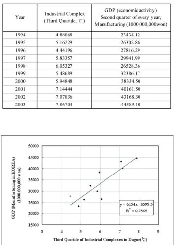
The GDP in the second quarter of each year for the manufacturing industries and the third-quartile values of the combined industrial complexes in April or May were compared (Table 5). Regression analysis (R2 = 0.7576) showed that there were significant consequences. (If the value in 1998 is excluded from the 10-year values R2 = 0.8482.)
Table 5. Third-quartile(℃) Tn values of the combined industrial complexes and manufacturing industries’
GDP in the second quarter of each year.
Figure 7. Regression analysis of the surface temperature of the industrial complexes and GDP.
5. CONCLUSION
This study was intended to elucidate the characteristics of surface temperatures in manufacturing areas that had undergone change due to economic conditions. Daegu was selected as the study region, and band 6 of Landsat was used to calculate surface temperatures in 1994~2003.
For temporal and spatial comparisons, surface temperatures in some playgrounds in Daegu were surveyed and Tp,y values were determined to calculate normalized Tn,y values.
Forty-five factories running textile businesses in the dyeing industrial complexes of Daegu were selected, and changes in surface temperatures at the factories were analyzed. The factories were divided into sections to evaluate temperature increases or decreases in the sections. When compared to the number of factories in the dyeing industrial complexes that had actually closed or leased facilities to others, there were significant differences. A comparison of the quartile values of the combined dyeing industrial complexes with the values from individual factories showed that using third-quartile
Year Industrial Complex (Third Quartile, ℃)
GDP (economic activity) Second quarter of every year, M anufacturing (1000,000,000won)
1994 4.88868 23434.12
1995 5.16229 26302.86
1996 4.44196 27816.29
1997 5.83357 29941.99
1998 6.05327 26528.36
1999 5.48689 32386.17
2000 5.94848 38334.50
2001 7.14444 40161.50
2002 7.07836 43168.30
2003 7.86704 44589.10
values would be appropriate for excluding the influence of support facilities that make up parts of the industrial complexes (e.g., road and street trees) and so reflecting the actual state of the industrial complexes. The representative values of the individual industrial complexes were then established. Temperatures increased by around 3℃ in 2003 compared to 1994. Finally, the third-quartile values of the combined industrial complexes of Daegu were compared with the manufacturing industries’ GDP. The results showed positive correlations, indicating that surface temperatures in industrial areas reflect the industrial economy.
Through additional studies on comparisons between individual factories and differences between types of businesses, the scope of this investigation will be expanded so that the results can be more widely applied.
The exploration of temporal and spatial changes in surface temperatures can be applied to other areas. If correlations between data from remote sensing and social, economic and cultural data can be derived, many applied studies could be conducted.
If surface temperatures increased along with industrialization in the past, we should now be promoting sustainable growth that will not increase national temperatures. If remote sensing technologies and GIS are applied to this effort, it will become possible to manage national lands while addressing problematic areas.
Temperature management through AWS meteorological data or site measurements has limitations. A strategy to continue monitoring and managing surface temperatures through remote sensing is required.
References from Journals:
Chander, G., Markham, B., 2003. Revised Landsat-5 TM radiometric calibration procedures and postcalibration dynamic ranges. IEEE Transaction on Geoscience and Remote Sensing, 41(11), pp. 2674-2677.
Chatterjee, R.S., 2006. Coal fire mapping from satellite thermal IR data – A case example in Jharia Coalfield, Jharkhand, India. ISPRS Journal of Photogrammetry &
Remote Sensing, 60, pp. 113-128.
Griend, A. A and M. Owe, 1993. On the relationship between thermal emissivity and the normalized difference vegetation index for natural surfaces. International Journal of Remote Sensing, 14(6), pp.1119-1131.
Lagio, E., Vassilopoulou, S., Sakkas, V., Dietrich, V., Damiata, B.N., Ganas, A., 2007. Testing satellite and ground thermal imaging of low-temperature fumarolic fields: The dormant Nisyros Volcano (Greece). ISPRS Journal of Photogrammetry & Remote Sensing, 62(6), pp.
447-460.
Lambin, E. F., D. Ehrlich, 1996. The surface temperature-vegetation index space for land cover and
land-cover change analysis. International Journal of Remote Sensing, 17(3), pp. 463-487.
Lee, Kwang-Jae, Jo, Myung-Hee, 2004. Analysis of urban surface themperature distribution properties using spatial information technologies. Korean Journal of Remote Sensing, 20(6), pp. 397-408.
Prakash, A., Gens, R., Vekerdy, Z, 1999. Monitoring coal fires using multi-temporal night-time thermal images in a coalfield in north-west China. International Journal of Remote Sensing, 20(14), pp. 2883-2888.
Xian, G., Crane, M., 2006. An analysis of urban thermal characteristics and associated land cover in Tampa Bay and Las Vegas using Landsat satellite data. Remote Sensing of Environment, 104, pp. 147-156.
Nasa, 1998, Landsat 7 Science Data User Handbook http://landsathandbook.gsfc.nasa.gov/handbook.html (accessed 28 September 2009)
Korean Statistical Information Service http://www.kosis.
kr (accessed 28 September 2009)