Frequently Occurred Information Extraction from a Collection of Labeled Trees
백 주 련* 남 정 현** 안 성 준*** 김 응 모****
Juryon Paik Junghyun Nam Sung-Joon Ahn Ung Mo Kim 요 약
트리 데이터로부터 유용한 정보들을 추출하는 가장 일반적인 방식은 빈번하게 자주 발생하는 서브트리 패턴들을 얻는 것
이다. XML 마이닝, 웹 사용 마이닝, 바이오인포매틱스, 네트워크 멀티캐스트 라우팅 등 빈번 트리 패턴 마이닝은 여러 다양한
영역에서 광범위하게 이용되고 있기 때문에, 해당 패턴들을 추출하기 위한 많은 알고리즘들이 제안되어 왔다. 하지만, 현재까 지 제안된 대부분의 트리 마이닝 알고리즘들은 여러 가지 심각한 문제점들을 내포하고 있는데 이는 특히 대량의 트리 데이터 집합을 대상으로 했을 때는 더 심각해 진다. 주요하게 발생하는 문제점들로는, (1) 계층적 트리 구조의 데이터 모델링, (2) 후보 군 유지를 위한 고비용 계산, (3) 반복적인 입력 데이터 집합 스캔, (4) 높은 메모리 의존성이 대표적이다. 이런 문제점들을 발생하게 하는 주요 원인은, 대부분의 기존 알고리즘들이 apriori 방식에 근거하고 있다는 점과 후보군 생성과 빈발 횟수 집계
에 anti-monotone 원리를 적용한다는 점에 기인한다. 언급한 문제들을 해결하기 위해, 본 저자들은 apriori 방식 대신
pattern-growth 방식을 기반으로 하며, 빈번 서브트리 추출 대신 최대 빈번 서브트리 추출을 목적으로 한다. 이를 통해 제안된
방법은, 빈번하지 않은 서브트리들을 제거하는 과정 자체를 배제할 뿐만 아니라, 후보군 트리들을 생성하는 과정 또한 전혀 수행하지 않음으로써 전체 마이닝 과정을 상당히 개선한다.
ABSTRACT
The most commonly adopted approach to find valuable information from tree data is to extract frequently occurring subtree patterns from them. Because mining frequent tree patterns has a wide range of applications such as xml mining, web usage mining, bioinformatics, and network multicast routing, many algorithms have been recently proposed to find the patterns.
However, existing tree mining algorithms suffer from several serious pitfalls in finding frequent tree patterns from massive tree datasets. Some of the major problems are due to (1) modeling data as hierarchical tree structure, (2) the computationally high cost of the candidate maintenance, (3) the repetitious input dataset scans, and (4) the high memory dependency. These problems stem from that most of these algorithms are based on the well-known apriori algorithm and have used anti-monotone property for candidate generation and frequency counting in their algorithms. To solve the problems, we base a pattern-growth approach rather than the apriori approach, and choose to extract maximal frequent subtree patterns instead of frequent subtree patterns. The proposed method not only gets rid of the process for infrequent subtrees pruning, but also totally eliminates the problem of generating candidate subtrees. Hence, it significantly improves the whole mining process.
☞ KeyWords : Tree mining, Maximal frequent subtree, Embedded tree, Pattern-growth method, 트리 마이닝, 최대 빈번서브 트리, 임베디드 트리, 패턴-성장 방식
* 정 회 원 : 성균관대학교 정보통신공학부 연구교수 [email protected]
** 정 회 원 : 건국대학교 컴퓨터응용과학부 조교수 [email protected]
*** 정 회 원 : 성균관대학교 정보통신공학부 부교수 [email protected]
**** 정 회 원 : 성균관대학교 정보통신공학부 교수 [email protected]
1. INTRODUCTION
1.1 MOTIVATION
One of the most general approaches for modeling
[2009/03/06 투고 – 2009/03/13 심사 – 2009/04/28 심사완료]
☆ 이 논문은 2009년도 정부(교육과학기술부)의 재원으로 한국 과학재단의 지원을 받아 수행된 연구임(No. 2009-0075771)
complex structured data is to prescribe the data with tree structure. In the database area [1, 2], XML documents are rooted trees where the nodes represent elements or attributes and the edges represent element-subelement and attribute-value relationships.
In Web traffic mining, access trees are used to represent the access patterns of different users [3]. In the analysis of molecular evolution, an evolutionary tree is used to describe the evolution history of certain species [4]. In computer networking, multicast trees are used for packet routing [5].
With the ever-increasing amount of available tree data, the ability to extract valuable information from them becomes increasingly important and desirable.
However, the problem of finding information on tree data has not been extensively studied, in spite of its applicability to a variety of problems. The first step toward finding information from trees is to mine the subtrees frequently occurring in the trees. Frequent subtrees in a database of trees provide useful knowledge in many cases such as gaining general information of data sources, mining of association rules, classification as well as clustering, and helping standard database indexing [6]. However, the discovery of frequent subtrees appearing in a large-scaled tree dataset is not an easy task. As observed in Chi et al's paper [7], due to combinatorial explosion, the number of frequent subtrees usually grows exponentially with the size (number of nodes) of the tree and, therefore, mining all frequent subtrees becomes infeasible.
A more practical and scalable alternative is thus required, which is the discovery of maximal frequent subtrees. A maximal frequent subtree is a frequent subtree for which none of its proper supertrees are frequent, and the number of them is much smaller than that of frequent subtrees. However, mining maximal frequent subtrees is still in the immature
stage and needs to be further researched, compared to the substantial achievements in mining frequent subtrees. Most existing researches on maximal frequent subtrees are inherently complex and cause some computational problems.
1.2 RELATED WORK
The most popular approaches to find useful information from trees are either apriori-based[8] or frequent-pattern-growth(FP)-based[9]. The algorithms based on the former extract frequent subtrees by the well known anti-monotone property: every non-empty subtree of a frequent tree is also frequent, for candidate-generate-and-test. Since it provides significant reduction of the size of candidate sets and leads to good performance gain, various techniques have been applied to improve their efficiency [10, 11, 12, 13]. They are efficient and scalable when short patterns are usually extracted from sparse datasets. What if datasets are dense and there are a lot of long patterns? That may degrade mining performance dramatically because a large number of candidates need to be generated and tested.
To solve the problems, FP-growth method is extended to mine tree patterns, which avoids the generation of candidates in support of the construction of concise in-memory data structures that preserve all necessary information, recursively partition an original database into several conditional databases and search for local frequent subtrees to assemble larger global frequent subtrees. However, it is not trivial work for trees because of two major obstacles: one is to test efficiently whether a pattern is a subtree of a given tree in a dataset. The other is to determine a good tree growing strategy and avoid tree redundancy. The algorithm XSpanner [14] has been recently presented to generate frequent patterns without explicit candidate generation, however, its recursive
projections of a dataset may cause a lot of pointer cashing and bad cache behavior.
The goal of the above mentioned algorithms is to discover all frequent subtrees from a database of trees. However, as observed in Chi et al's papers [13], the number of frequent subtrees usually grows exponentially with the tree size, therefore, mining all frequent subtrees becomes infeasible for a large number of trees. The algorithms presented by Xiao et al. [15] and Chi et al. [16] attempt to alleviate the huge amount of frequent subtrees by finding and presenting to end-users only the maximal frequent subtrees. The former uses a new compact data structure, FST-Forest, to store compressed trees, representing the trees in a database. Nevertheless, the algorithm uses post-processing techniques that prune away non-maximal frequent subtrees after discovering all the frequent subtrees. Therefore, the problem of the exponential number of frequent subtrees still remains. The latter directly aims at closed and maximal frequent subtrees only.
However, it bases on the enumeration trees, which is one of branches of apriori techniques. Therefore, this algorithm may have the potential problem if a dataset is dense and there are a lot of long patterns.
Handling the maximal frequent subtrees is an interesting challenge, though, and represents the core of this paper.
2. PROBLEM DEFINITIONS
General tree concepts A rooted tree is directed acyclic graph satisfying (1) there is a special node called the “root” that has no entering edges, (2) every other node has exactly one entering edge, and (3) there is a unique path from the root to each node. A tree is a labeled tree if there exists a labeling function that assigns a label to each node of
a tree. Let T = (r, N, E, L) be a rooted labeled tree, where r ∈ N is the root node, N is a set of nodes, E is a set of edges, and L is a labeling function which maps each node of T to one of labels in a finite set L = {l1, l2 ... li}; for any node v ∈ N, L(v) assigns the label of v. For brevity, in the remaining of this paper, unless otherwise specified, we call a rooted labeled tree as simply a tree.
Embedded Subtree Given a tree T = (r, N, E, L), we say that a tree S = (r', NS, ES, L') is included as an embedded subtree of T, denoted S ≾ T, iff (1) NS ∈ N, (2) for all edges (u, v) ∈ ES such that u is the parent of v, u is an ancestor of v in T, (3) the label of any node v ∈ NS, L'(v) = L(v). The tree T must preserve ancestor relation but not necessarily parent relation for nodes in S.
Support and frequent subtree The primary goal of mining some set of data is to provide information often occurred in a dataset. However, it is not straightforward in the case for trees unlike the case for traditional item data.
Let D = {T1, T2, …, Ti} be a set of trees and |D|
be the number of trees in D, where 0 < i ≤ |D|.
Given D and a tree S, the frequency of S with respect to D, freqD(S), is defined as ΣTi∈D freqTi(S) where freqTi(S) is 1 if S is a subtree of Ti and 0 otherwise. The support of S with respect to D, supD(S), is the fraction of the trees in D that have S as a subtree. That is, supD(S) = freqD(S) / |D|. A subtree is called frequent if its support is greater than or equal to a minimum value of support specified by users or applications. This user-specified minimum value is often called the minimum support (minsup or σ). The problem of mining frequent subtrees is defined as to uncover all pattern trees S, such that supD(S) = ΣTi∈D freqTi(S) / |D| ≥ minsup.
However, the discovery of frequent subtrees appearing in a large set of trees is not easy task to
do. The combinatorial time for subtree generation becomes an inherent bottleneck of frequent subtree extraction and it causes that finding all frequent subtrees is impossible.
Given some minimum support σ, a subtree S is called maximal frequent with respect to D iff it satisfies the following conditions: (1) the support of S is not less than σ, i.e., supD(S) ≥ σ. (2) there exists no any other σ-frequent subtree S' with regard to D such that S is a subtree of S'.
There are fewer maximal frequent subtrees compared to the number of frequent subtrees. In addition, by uncovering only maximal frequent subtrees, we do not lose other frequent information by the fact that the set of maximal ones subsumes all frequent subtrees.
3. THE PROPOSED ALGORITHM
In this section, we introduce a new pattern-growth algorithm SEAMSON (Scalable and Efficient Algorithm for Maximal frequent Subtrees extractiON) based on its interesting definitions and important features. The initial version of SEAMSON was presented in [17, 18].
3.1 LABEL PROJECTION
Finding frequently occurred subtrees is virtually to discover the subtrees whose nodes are labeled by frequently appeared labels in a given tree database D and, therefore, scanning database time to find out how many times each label has been used in D is one of the time consuming part in mining trees.
Trees are usually stored in D according to their relating documents and each document is treated as a transaction. That is document-driven layout. In such layout, the whole trees are scanned every time whenever frequency is computed for each label and,
thus, it requires O(|D||Tavg||L|) time complexity to get the frequencies of whole labels, where |D| is a total number of trees, |Tavg| is an average number of nodes of a tree, and |L| is a number of distinct labels. It is not serious problem when the number of |D| and
|Tavg| are reasonably small. It may hinder the computation, however, if both values are large, and actually in real world, two factors are large.
What if the database has been organized in a label-driven layout? A label itself plays the key role which is usually performed by tree or transaction indexes. All trees in D are reorganized according to labels. During scan of the trees in D, all nodes with the same label are grouped together. The nodes composed of the same tree form a member of the group and the number of members actually determines the frequency of the given label; the maximum number of members is a number of trees in D, which is called label-projection. After all labels are projected, the document-driven layout is changed into label-driven layout in which the time complexity to check labels' frequency requires at most O(|L||D|). If hash-based search is used, the complexity is reduced up to O(|D|).
Definition 1 (label list) Let l be a label in L.
During pre-ordered scanning trees, tree indexes and node indexes which are projected by l construct a single linked list. It is called a label list and the label list for a given label l is denoted l-list.
The structure of a label list is similar to that of a linked list in that it has a head and a body. The only difference is the formation and functionality of the head. The head of a label list points the first object in a body just like the ordinary head of a linked list.
Along with the indication, the head of a label list gives information on which node indexes have been
mapped to a projected label. The body of a label list follows immediately its corresponding head. The main concerns of a body are to evaluate how many trees have the key in its paired head and to find parents positions of the nodes in the head. The former is for dealing with frequencies of each label, while the latter is for handling the hierarchical information of the label. To achieve such intentions, the structure of a body is a sequence of members which is arranged in a linear order. Each member is an object with one key field, one link field pointing to the next member, and one satellite data field.
As a key, a tree index number is used, which means that the label in a corresponding head has been assigned to the nodes of the tree. During the database scan, the member is generated and inserted into bodies of label lists. The newly inserted member is added to the end of a proper body and the pointer field of its previous member points this new member. The body of a label list provides the method we can judge in how many trees have the label of a current label list, that is the number of members in a body and we define it as size of a label list.
Assume T1, T2, and T3 in D are the trees whose at least one node is labeled by l. The nodes having l in each tree are: na ∈ T1, nb, nc ∈ T2, and nd 1
∈ T3. A number of members of l-list are three because 3 trees include the label. The l-label projection, l-list, is〈 (pa, T1, →), (pb pc, T2, →), (pd, T3, ε) 〉, where pa, pb, pc, pd are parent node indexes, → means a pointer to a next member, and ε means an empty pointer.
Definition 2 (label dictionary) The constructed label lists are collected and stored in the memory.
Whenever a label is given, a corresponding label list is retrieved and the count of its members is returned.
Due to its activity, the collection is named as label dictionary, denoted Ldic.
As infrequent single-node trees are eliminated in conventional approaches, the label lists which do not confirm a given threshold δ, δ = σ * |D|, must be pruned from Ldic, because the initial Ldic is analogous to a set of all single-node trees of D.
Figure 1 shows an depicted example of how Ldic
and its label lists are constructed and managed from the database D. For easy distinction between nodes of different trees, we assign unique consecutive indexes in pre-order traversal. The bodies of lists decide the frequencies of corresponding labels. For instance, the label A does not satisfy the given minsup which is set ⅔ because it has only 1 member in the body of A-list.
Definition 3 (frequent label list) Given a label list for l, l-list ∈ Ldic, let |l-list| be a number of its members. l-list is said to be a frequent label list iff it satisfies the following conditions: (1) |l-list| ≥ δ (2) for each member, every parent index p in it, the label of p, L(p), has been projected and has L(p)-list. (3) |L(p) -list| ≥ δ.
T1 T2 T3
A
C
D B E
F
G F
1 2 5
3 7
6
4 8
C
B
D E
F
F G
9 12
10 14
13
11 15
C
C D B E
B E
F G
F
16 22
17 23 25
18 20
19 21
24
1 1 2,9,(16,17) 2,9,(16,17) 3,10,22 3,10,22
5,12,(18,23) 5,12,(18,23) (6,8),(11,13),(19,24) (6,8),(11,13),(19,24) A
C D G B F E
4,15,21 4,15,21
7,4,(20,25) 7,4,(20,25)
T1 ε
0 T1 ε
0 T1 1 T1 1
T1 2 T1 2
T1 3 T1 3
T1 2 T1 2
T1 5,7 T1 5,7
T1 2 T1 2
T2
0 T2
0 T2
9 T2
9 T2 14 T2 14
T2
9 T2
9 T2 10,12 T2 10,12
T2
9 T2
9
T3 ε 0,16 T3 ε 0,16
T3 ε 16 T3 ε 16
T3 ε 20 T3 ε 20
T3 ε 17,16 T3 ε 17,16
T3 ε 18,23 T3 ε 18,23
T3 ε 17,16 T3 ε 17,16 A-list
head part body part
(Figure 1) Original tree database and its label dictionary Ldic
A label list is said to be projected from a frequent label iff the first condition is satisfied. Since our approach is inspired by the pattern growth algorithms, the label lists whose projected labels do not confirm the first condition cannot be further grown. Even a label list is projected from a frequent label, it is still not clear if the list is a frequent label list or not, because of the structural uniqueness of a label list which is one of the key factors in allowing SEAMSON not to generate any subtrees.
The parent indexes in members should have frequent labels in order the subtrees with size 2 to be frequent, and this is checked by the second and third condition of Definition 3. However, it rarely happens that parent index also has frequent label. In that case, such a parent index whose label is not frequent can be switched to either one of its ancestors which label is frequent, or the root, because SEAMSON cares embedded subtrees. Some means to manage parent indexes in members is required to check the frequency of and to switch them, which makes label lists be frequent.
3.2 CANDIDATE HASH TABLE
Before acquiring frequent label lists, the method to make them must be provided, which is the distinctive feature of SEAMSON and make it differentiate from previous approaches. To this end, the label lists whose projected labels do not satisfy the condition (1) of the definition 3 are excluded from Ldic (now, the current Ldic is denoted Ldicf
) and form a special hash table named Candidate Hash Table, TC, whose purpose is to determine if a given node index has a frequent label or not. If its label is found in the table, it means that the label is infrequent because its label list is not in Ldicf. The parent indexes of members in Ldicf are verified and switched to fulfill the last two conditions of the
definition. TC is composed of node indexes, labels of the nodes, and label lists, where keys are labels and their values which are label lists are returned by a hash function H(label). Note that the input of the table is node indexes which are mapped to their proper labels by L(n).
Theorem 1 It is infeasible that an identical label list is included in both Ldicf and TC.
Proof. Assume a label list, say l-list, exists in both Ldicf
and TC. This situation directly creates conflict; It is reasonable l-list has frequent label if it is in Ldicf. Hence, it is never excluded from Ldicf, which means there is no chance for the list to be in TC. On the contrary, once l-list is in TC, it indicates the label l didn't satisfy a given σ. The label list had to be definitely pruned from Ldic. Therefore, any label list generated from a label in L is contained in either Ldicf
or TC.
It is easily determined by TC if the label of a given parent index has projected as one of label lists in Ldicf
, then, what about the switching in case the label is in TC. As the required method we define the following.
Definition 4 (closest frequent ancestor) Given an arbitrary label list in Ldicf
, any parent index p in its members is required to traverse its ancestors if L(p) is in TC. During the move toward the root, the ancestor index of p is searched what is the first ancestor whose label is not in TC. We call this ancestor closest frequent ancestor of p, denoted Λp.
Let l1-list (∈ Ldicf) is a current label list and
|l1-list| be m. Each member of its l1-list.b is required to undertake the following. Let any parent node index in members be p. Note that p’s nth ancestor is notated by pn (p0 is p itself). (1) Each p of a
member is associated to its label by L(p). (2) The obtained L(p) is given to TC. If L(p) is not found between keys, p has frequent label. Thus, p becomes the proper Λp, and the process is terminated.
Otherwise, p’s label is infrequent. (3) To uncover the desired location of L(p), the index is computed by H(L(p)). (4) According to H(L(p)), the value L(p)-list is returned. (5) Since the value is L(p)-list.b, it consists of several members. The node indexes in the members correspond to those of p1. (6) As backtracking, (1) to (4) is done against every p1 in the value. (7) The p1 whose label is found as the key of TC iteratively performs (3) through (6) until Λp1
is found. For all m members the steps (1) to (7) are performed to fill themselves with only closest frequent ancestors. What if a proper Λp is not acquired until end of backtracks? In such case, none of p's ancestors including p itself have frequent labels. That means the node index whose label is l1 has no parent node, and therefore, it becomes the root. Hence, Λp is set by 0 to indicate that ‘it is the root position’.
The figure 2 shows TC constructed simultaneously with Ldicf
(Here, Ldicf
is the same as Ldic on Figure 1, except that it does not contain A-list and C-list has been modified by the closest frequent ancestor.
A
key index value
1 node index
L(1) H(A) 00 TT11 εε
1 T1
1 T1 00 TT22 0, 160, 16 TT33 εε C-list 2,9,16,172,9,16,17
0 T1
0 T1
2 T1 2 T1 3 T1 3 T1 2 T1 2 T1 5, 7 T1 5, 7 T1
2 T1
2 T1
0 T2
0 T2
9 T2
9 T2
14 T2 14 T2
9 T2
9 T2
10,12 T2 10,12 T2
9 T2
9 T2
0, 16 T3 ε 0, 16 T3 ε
16 T3 ε
16 T3 ε
20 T3 ε
20 T3 ε
16,17 T3 ε 16,17 T3 ε 18,23 T3 ε 18,23 T3 ε 16,17 T3 ε 16,17 T3 ε C-list
D-list G-list B-list F-list E-list
2,9,16,17 2,9,16,17 3,10,22 3,10,22 4,15,21 4,15,21 5,12,18,23 5,12,18,23 6,8,11,13,19,24 6,8,11,13,19,24 7,14,20,25 7,14,20,25
TC
Ldicf 0 L(0) ?
(Figure 2) Discovery and replacement of Λ1
3.3 LABEL LIST EXTENSION The finally obtained Ldicf
contains all frequent label lists, which implicitly indicates the projected labels are all frequently occurred and every node index is mapped by one of them. Then, what about paths between nodes if the nodes are explicitly linked? In such case, the paths could possibly be frequent, however, that is not guaranteed because of the fact that a path is a sequence of edges. Let an edge e connect exactly two distinct nodes v1, v2
labeled by a and b, which is notated e = (v1, v2) = (L(v1), L(v2)) = (a, b). If e wants to be a frequently occurred edge, the labels a and b must be frequent labels. Hence, if a path wants to be a frequently appeared path, all edges forming the path should be frequently occurred. When let a path be p, it is composed of a finite number of edges; p = e1 e2… em. The path can also be expressed with labels because a path is a sequence of labels as shown on the above equations. Therefore, all the labels should be frequent in order the path to be frequent.
However, it is not guaranteed when edges between nodes are explicitly unveiled from Ldicf
, because only nodes and labels were considered to build the initial Ldic. During the read of label lists, edges are formed by joining a symbolic node whose label is the projected label and symbolic nodes of parent indexes’ labels in its members. Unveiling edges totally relies on every frequent label lists, because the symbolic nodes of parent indexes' labels have also their frequent label lists. The hidden paths between label lists are discovered by extending the node of a current label with the nodes of other label lists.
Definition 5 (label list extension) Given Ldicf, let a current label list be l-list and p be one of parent indexes in its members. For l-list, firstly a symbolic
node whose label is l is set and the node is prepared to join with its parent. The second symbolic node is set from the parent index p. Its label is easily obtained by L(p) and the corresponding L(p)-list is in Ldicf due to the definition 3. Consequently, the node labeled by l is joined to the node labeled by L(p). We call this operation label list extension and denote l ← L(p) where ‘←’ indicates the direction of parent to child.
Note that the extension is performed with labels not the node indexes. The node index is just used to get label or its corresponding label list. A symbolic node is created whenever a label requires it. The fundamental method is actually to extend label. The label list extension is committed to every label list in Ldicf. After completing the work of extension, the labels in head parts are connected each other via nodes. The structure of the result is a tree whose root is labeled by /. This tree contains all of potentially maximal frequent subtrees and thus is named Potentially Maximal Pattern tree (PMP-tree in short). The detailed is followed.
Two times of Ldicf scans are required. First, only head parts of label lists are scanned to determine how many symbolic nodes are needed. This number depends on |Ldicf| since head part exists per label.
The settled number of nodes are created and related by labels in head parts. During the first scan, the nodes are fixed and they are never changed because label list extension is performed on the basis of those nodes and PMP-tree is also derived from them.
These nodes are called seeds of PMP-tree. Each seed contains three fields; cnt field for edge frequency, and two pointer fields: prt and suc for parent node and successor node, respectively. The detailed roles of fields will be explained in the paragraph for second scanning.
Along with the determination of seeds, one table is constructed with labels and seeds. This table facilitates the traversal of PMP-tree by providing location information of seeds. Once a label is given to the table, its corresponding seed’s position in PMP-tree is retrieved. Since the table searches nodes based on labels, we name it Label Header Table, TL, and it is built simultaneously with seeds. TL is composed of two columns: label and seed# (location of seed).
The storage size required for saving the table is followed. Assuming a size of a single table record x and |Ldicf
| = M, the total required space is fixed at xM because seeds are created from the labels of all heads in Ldicf. It has a storage complexity of Θ(x|L|) time in the worst case, however, it is unusual that every unique label for D is frequent. Therefore, the actually necessary space to store TL is much smaller than the worst case, because of M ≪ |L|.
After finishing the first scan, total seven seeds are generated from the Ldicf
on Figure 2 and they are related their labels in TL via the seed# column. The current seeds have empty parents, empty successors, and 0 counters. Since not yet performed the label list extension, no relation is expected between seeds. To process label list extension over the seeds, Ldicf is scanned for the second time and last time. During this scanning period, the body parts in turn are analyzed, which have been skipped at the first scan.
The parent indexes of each member are spliced with the existing seeds by following steps: (1) Let a seed of a current reading label list, l-list, be sl associated with a label l in TL. (2) For a parent index p in a member of body of l-list, obtain a label of p by L(p). (3) According to Definition 3, the label L(p) forms a record of TL and is associated with one of seeds. (4) Look up the table TL to get the seed#
which corresponds to L(p); let the corresponding
seed be sL(p). (5) If sl has empty prt which means it is not yet linked with any parent node, the seed sL(p)
is the firstly appeared its parent. Hence, the seed# of sL(p) is stored in the prt of sl; this action directly perform sl ← sL(p). Also, the cnt of sL(p) is incremented by 1 because an edge between sl and sL(p) has been formed and it occurred. The value of cnt implies frequency of an edge which is formed between a current seed and a parent seed. Instead of incrementing the current seed’s cnt, we choose to increment the parent seed’s cnt because the parent seed is end point of an edge. Because making edge is completed by the parent seed, the information of edge frequency has to be kept in parent, which means “child seed and I occurred together as many as my cnt times”. Thus, we increment the edge frequency in parent seed.
It is trivial work to link sl to sL(p) when prt of sl
is empty. However, what if prt of sl is already preoccupied by another seed#, say sL(q)? There are two cases depending on whether sL(p) = sL(q) or not, and the step (5) in the previous paragraph is replaced by the following: (5-1) If sL(p) ← sL(q), the fact has to be taken into account that the seed sl has more than one parents with different labels. To cope with such situation, we add a successor at the end of the seed sl, or at the last successor if sl already has successors. Successor has exactly same structure as that of seed. Without using successors one child can have several parents and it causes the graph structure which requires NP-complete subtree decomposition.
In case of that sl has successors, the values in all prts of sl and its successors have to be compared with the seed# of sL(q). If not found the same value, sL(q) is another parent seed of sl, thus, a new successor for sl is attached at the end of successors and it is linked with sL(q). (5-2) In case of that sL(p)
is equal to the preoccupied prt value sL(q) or any one
of prt values in sl’s successors, cnt of sl or corresponding successor is incremented by 1.
Because the edge of between sl and sL(p) has been already made, the only work is to increase the frequency; the already existing edge corresponds either to sl ← sL(q) or to sl.suc ← sL(p) (6) The procedures from step (2) to (5-2) is repeated until all parent indexes in Ldicf are considered.
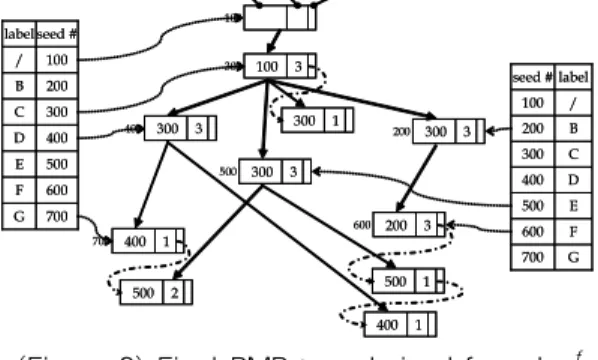
Figure 3 illustrates both the table TL and the derived PMP-tree from Figure 2. The currently obtained PMP-tree is composed of many edges which link between seeds or successors. Connecting nodes in a tree implies the extension of tree. The frequency of nodes is considered in PMP-tree, however, the frequency of edges is not guaranteed.
Therefore, frequency of an edge has to be considered to complete the PMP-tree. This is done by marking the counts of edges in the field cnt of each seed or successor. If s.cnt is less than a given threshold, s and its entering edge are not frequent. Thus, both are spliced out from a current PMP-tree. On the figure, only the edges with bold lines are remained edges in PMP-tree.
700 G
600 F
500 E
400 D
300 C
200 B
100 /
seed # label
700 G
600 F
500 E
400 D
300 C
200 B
100 /
seed #
label 100100
300 100 3 300 100 3
400 300 3
400 300 3 300300 11 500 300 3 500 300 3
200 300 3 200 300 3
600 200 3 600 200 3
500 1 500 1 400 1 400 1 700 400 1
700 400 1
500 2 500 2
prt cnt suc
G 700
F 600
E 500
D 400
C 300
B 200
/ 100
label seed #
G 700
F 600
E 500
D 400
C 300
B 200
/ 100
label seed #
(Figure 3) Final PMP-tree derived from Ldicf
4. EXPERIMENTS
We performed some experiments to evaluate the performance of SEAMSON algorithm using synthetic datasets. All experiments were done on a 2.2GHz
AMD Athlon 64 3500+ PC with 1GB main memory, running Windows XP operating system. All algorithms were implemented in Java. The synthetic datasets are generated by the tree generation program whose underlying ideas are inspired by Termier [19]
and Zaki [12]. The generator constructs a set of trees, D, based on some parameters supplied by a user, T:
the number of trees in D, L: the set of labels, f: the maximum branching factor of a node, d: the maximum depth of a tree, ρ: the random probability of one node in the tree to generate children or not, η: the average number of nodes in each tree in D.
We used the following default values for the parameters: T = 10,000, L = 100, f = 5, and d = 5.
In the following experiments, we first evaluate the scalability of our algorithm with varying minimum support as well as the number of trees T, while other parameters are fixed as: L = 100, f = 5, d = 5, ρ = 20%, η = 13.8. Second, we present the number maximal frequent subtrees under different minsup.
As the last experiment, the memory usage of SEAMSON is evaluated while minsup is 0.2% and 0.1%, where its characterized processes: constructing Ldic, finding closest frequent ancestors, and deriving PMP-tree, are especially evaluated for their memory consumption. In the figures of experiments, both X- and Y-axis are drawn on a logarithmic scale for the convenience of observation.
100 101 102 103
10-4 10-3
10-2 10-1
100 101
Running time (sec)
Minimum Support (%)
T = 10000 T = 15000
(a) support vs. time
0 20 40 60 80 100 120 140 160 180 200 220 240
1⋅103 2⋅103 3⋅103 4⋅103 5⋅103 10⋅103 15⋅103
Running Time (sec)
Number of Input Trees (T) minsup = 0.2%
minsup = 0.15%
minsup = 0.1%
(b) input trees vs. time
0 10 20 30 40 50 60 70 80 90
10-4 10-3
10-2 10-1
100 101
Number of Maximal Frequent Subtrees(trees)
Minimum Support(%)
T=10000 T=15000
(c) number of maximal frequent subtrees
0 5 10 15 20 25 30 35 40
1⋅103 2⋅103 3⋅103 4⋅103 5⋅103 10⋅103 15⋅103
Memory Usage (MB)
Number of Trees in a Dataset (T) Constructing L+dic
Finding cfa Deriving PMP-tree
(d) memory usage per each process
(Figure 4) Scalability and memory consumption of SEAMSON
From Figure 4(a), we can find that the running time increases when T increases, however, both running times are rarely affected by the decrease of the minimum support. With minsup becoming