The Impact of Investor Sentiment on Energy and Stock Markets-Evidence : China and Hong Kong

Abstract

Purpose - The oil price affects company value, which is the present value of the expected cash flow, by affecting the dis- count rate and cash flow. This study examines the nonlinear re- lationships between oil price and stock price using the AlphaShares Chinese Volatility Index as the threshold.

Research design, data, and methodology – Data comprise daily closing values of the Shanghai Stock Exchange Composite Index, Shenzhen Stock Exchange Composite Index, and Hang Seng Index of ChinaWest Texas Intermediate crude oil spot price and AlphaShares Chinese Volatility Index from May 25, 2007 to May 24, 2012. The Threshold Error Correction Model is used.

Results - The results demonstrate different relationships be- tween the stock price index and oil price under different investor sentiments; however, the stock price index and oil price could adjust to a long-term equilibrium the long-term causality tests between them were all significant.

Conclusions - The relationship between the WTI and HANG SENG Index is more significant than the Shanghai Composites Index and Shenzhen Composite Index, when using the AlphaShares Chinese Volatility Index (ASC-VIX) as the investor sentiment variable and threshold.

Keywords: Oil Price, Stock Price, Investor Sentiment, TECM, China, Hong Kong.

JEL Classifications: G00, G10, F00.

1. Introduction

Oil price affects economy, such as output, employment, in- flation, interest rate, consumption, economic growth and re-

* Corresponding Author, Assistant Professor, Department of Applied Financial, Hsiuping University of Science and Technology, Taiwan.

E-Mail: konah@mail.hust.edu.tw.

cession, since oil is a major production factor (Hamilton, 1983;

Bernake, 1983; Gisser and Goodwin, 1986; Chen, Roll, and Ross, 1986l Pindyck, 1991; Rotemberg and Woodford 1996;

Jones and Kaul, 1996; Sadorsky, 1999; Park and Ratti, 2008, Apergis and Miller, 2009; El Dedi Arouri, Jouini, and Nguyen, 2011). However, the impact of oil shock on economy downturn is still inclusive (Hooker, 1966). Literature shows the nonlinear relationships between oil prices and the economy (Lee et al., 1996; Hamilton, 1996; Hungtinton, 1998). The increase of oil price has bigger impact on economy downturn than the de- crease of oil price on economy growth.

Oil price affects company value since the company value is the present value of the expected cash flow. Therefore, oil price affects stock price by two factors, discount rate and cash flow.

Inflation rate will increase if oil price increases. This will lead to higher interest rate and discount rate. Stock price has negative relationships with discount rate. However, investors receive two kinds of returns from stock investment, dividend and capital gain. A positive expected dividend gain plus expected capital gain tends to have the stock price increase. Therefore, high in- flation may not lead to lower stock price. During high inflation period, return from saving account could be negative. It is pos- sible that the stock price increases during high oil price and high inflation period if the expected capital gain is high. Some empirical studies show the negative relationship between oil price and stock price (Kling, 1985; Jones and Kaul, 1996; Faff and Brailsford, 1999; Papapetrou, 2001; Sadorsky, 2001;

Driesprong, Jacobsen and Maat, 2008). However, some literature shows weak or no relationship between oil price and stock price (Huang et al, 1996; El-Sharif et al, 2005; Cong, Wei, and Liao, 2008). Oil price shocks have negative impacts on the oil import countries, and have positive impacts on the oil export countries (Park and Ratti, 2008). Oil price increase has positive impact on the oil and gas company stocks (Sadorsky, 2001).

The conditional expected excess market return and the condi- tional variance of the market are related based on the inter- temporal asset pricing model (Merton, 1973). However, the con- ditional variance is unobservable (Ghysels et al., 2005). This makes it hard to have a unified conclusion about the relation- ship between the conditional expected excess return and condi- tional variance. Literature show positive relationships between Print ISSN: 1738-3110 / Online ISSN 2093-7717

doi: 10.13106/jds.2014.vol12.no3.75.

The Impact of Investor Sentiment on Energy and Stock Markets-Evidence : China and Hong Kong

11)

Liang-Chun Ho*

Received: January 14, 2014. Revised: February 09, 2014. Accepted: March 17, 2014.

conditional expected excess return and conditional variance (French et al, 1987; Ghysels et al, 2005l; Guo and Whitelaw, 2006; Guo and Neely, 2008 and Lundblad, 2007) and negative and weak relationships between conditional expected excess re- turn and conditional variance (Baillie and DeGennaro, 1990;

Campbell and Hentschel, 1992; Brandt and Kang, 2004; Goyal and Santa-Clara, 2003; Lettau and Ludvigson, 2003; and Li et al. 2005). VIX index, which contains information about future ex- cess market return and variance, can be used to estimate the conditional variance (Day and Lewis, 1992; Blair et al., 2001;

Guo and Whitelaw, 2006; Banerjee et al., 2007; Kanas, 2012).

The Chicago Board Options Exchange Volatility Index (VIX) is an indicator of future 30 days U.S. stock market volatility. It is considered to be an investor fear gauge or investor sentiment in the U.S. stock markets. Literature shows that VIX is called the investor fear gauge. High levels of VIX coincide with high de- grees of market turmoil in the U.S. (Whaley, 2000). Some liter- ature shows high level of VIX index followed by positive future stock market return and low level of VIX index followed by neg- ative future stock market return (French et al., 1987; Fleming et al., 1995; Giot, 2005; Guo and Whitelaw, 2006). This indicates that oversold market tends to have high level VIX index.

Oversold stock market leads to a positive relationship between VIX index and future stock market return (Giot, 2005). Some lit- erature shows negative contemporaneous relationship between VIX changes and stock market return (Fleming et al., 1995).

This indicates that VIX index and stock market index have in- verse relationship. Since VIX index is mean reverting, a neg- ative contemporaneous relationship between VIX index changes and stock market returns may be followed by a positive relation- ship between VIX index changes and past stock market returns (Guo and Wohar, 2006). Some literature shows that the VIX in- dex and stock market return have asymmetric relationship. An increase of VIX index from a negative stock market return is bigger than the decrease of VIX index from a similar positive stock market return (Schwert, 1990; Flemming et al., 1995). VIX index has significantly suppressing effect on oil prices in the long run (Sari, Soytas and Hacihasanoglu, 2011). It will be inter- esting to see if VIX can also be used as an investor sentiment in Chinese market. AlphaShares Chinese Volatility Index (ASC-VIX) is used in this paper. In addition, from our knowl- edge, there is no paper that uses the VIX index as the thresh- old to study the nonlinear relationships between oil price and stock price. This paper studies the nonlinear relationships be- tween oil price and stock price by using the AlphaShares Chinese Volatility Index (ASC-VIX) as the threshold.

This paper is organized as follows. Section 2 presents the data used in the study. Section 3 briefly describes the empirical methodology. Section 4 shows the empirical results and section 5 concludes this study.

2. Data

Daily closing values of Shanghai Stock Exchange Composite

Index (SSE Composite Index), Shenzhen Stock Exchange Composite Index (SZSE Composite Index) and Hang Seng Index (HSI) of China, West Texas Intermediate (WTI) crude oil spot price, and AlphaShares Chinese Volatility Index (ASC-VIX) are used in this study. The research period is from May 25, 2007 to May 24, 2012. And data of the variables is taken from Taiwan Economic Journal (TEJ), Energy Information Administration (EIA) and Bloomberg

¹⁾

.

AlphaShares China Volatility Index is a measurement of the implied volatility of options on major China equity indexes.

Chicago Board Option Exchange Volatility Index (VIX) is the market volatility expectation. AlphaShare Chinese Volatility Index is a measurement of the implied volatility of options on major China equity indexes, including Hang Seng Index and FTSE/Xihhua 25 index. It is calculated by a formula similar to the Chicago Board Options Exchange Volatility Index (VIX).

AlphaShares China Volatility Index can be used to represent the market volatility expectation of Chinese market.

Figures 1 to 8 show the historical chart for each variable.

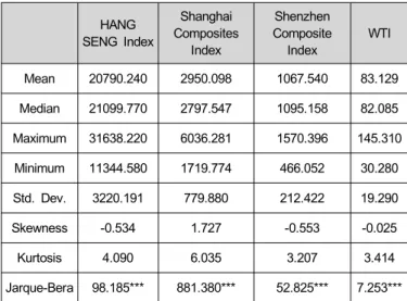
Table 1 presents some descriptive statistics, such as mean, standard deviation, maximum, minimum, skewness, kurtosis, and Jarque-Bera value. Among three stock indices and WTI, WTI has the smallest standard deviation and HANG SENG Index has the largest standard deviation. About skewness statistics, only SHANGHAI COMPOSITE Index is right-tailed. And the Jarque-Bera tests show that all variables reject the null hypoth- esis of normal distribution at 1% significance level.

<Table 1> descriptive statistics of Variables SENG Index HANG

Shanghai Composites

Index

Shenzhen Composite

Index WTI

Mean 20790.240 2950.098 1067.540 83.129

Median 21099.770 2797.547 1095.158 82.085 Maximum 31638.220 6036.281 1570.396 145.310 Minimum 11344.580 1719.774 466.052 30.280 Std. Dev. 3220.191 779.880 212.422 19.290

Skewness -0.534 1.727 -0.553 -0.025

Kurtosis 4.090 6.035 3.207 3.414

Jarque-Bera 98.185*** 881.380*** 52.825*** 7.253***

1. ***, **, and * denote the significant levels at 1%, 5%, and 10%.

1) http://www.bloomberg.co.jp/apps/quote? T=jp09/quote.wm&ticker =

ASCNCHIX: IND

<Figure 1> 2007/5/25-2012/5/24 West Texas Intermediate crude oil <Figure 2> Return of West Texas Intermediate crude oil

<Figure 3> 2007/5/25-2012/5/24 Shanghai Composites Index <Figure 4> Return of Shanghai Composites Index

<Figure 5> 2007/5/25-2012/5/24 Shenzhen Composite Index <Figure 6> Return of Shenzhen Composite Index

<Figure 7> 2007/5/25-2012/5/24 HANG SENG Index <Figure 8> Return of HANG SENG Index

3. Research Method

3.1. Nonlinear Unit Root Test: Kapetanios, Shin, and Snell (KSS) Test

The Augmented Dickey-Fuller test (Sims, 1988) and Phillips-Perron test (Phillips and Perron, 1988) are used for the linear unit root test. The ADF and PP tests are for the null hy- pothesis that a time series is I(1). The Kwiatkowski, Phillips, Schmidt and Shin (1992) KPSS test is usedto reinforce the re- sults from ADF and PP tests. The KPSS stationary test is for the null hypothesis that a time series is I(0).The Kapetanios, Shin, and Snell (2003) KSS nonlinear unit root test is used for the nonlinear stationary test.

The KSS test isto detect the presence of non-stationary against a nonlinear but globally stationary exponential smooth transition autoregressive (ESTAR) process. The model is ex- pressed as follows.

t t t

t

X X

X = α − − γ + ε

Δ

−1

{ 1 exp(

²₋₁

)} (1)

where ^X

^t

is the time series data. ε is an independently iden-

^t

tically distributed, iid, error term with zero mean and constant variance. And γ ≥ 0 is the transition parameter of the ESTAR model and governs the speed of transition. Under the null hy- pothesis, ^X

^t

follows a linear unit root process. And ^X

^t

follows a nonlinear stationary ESTAR process under the alternative hypothesis. One shortcoming in this framework is that the pa- rameter γ is not identified under the null hypothesis. Replacing

)}

exp(

1

{ − − γ X

_t²₋₁

in equation (1) by a first-order Taylor series ex- pansion around γ = 0, the following auxiliary model can be de - rived (Kapetanios, Shin, and Snell, 2003).

T t X

X c

X

t

k i

i t t i

t

, 1 , 2 , K

1 3

1

+ Δ + =

+

=

Δ ∑

=

−

β

−

ν

θ (2)

⎩ ⎨

⎧

<

= 0 :

0 :

1 0

θ θ H H

(3)

Under this framework, the null hypothesis and the alternative hypothesis are expressed as θ ^{= 0} (non-stationary) against

< 0

θ (nonlinear ESTAR stationary). If it is rejected then it is nonlinear stationary. If it cannot be rejected then it is non-stationary.

3.2. Threshold Autoregressive / Momentum-Threshold Autoregressive cointegration tests

Nonlinear asymmetric adjustment processes may exist be- tween the nonstationary variables in the linear models. Nonlinear models are better solutions to capture nonlinear cointegration re- lationship between variables. (Enders and Granger, 1998;

Enders and Siklos, 2001). Threshold Autoregressive (TAR)/

Momentum-Threshold Autoregressive (MTAR) cointegration tests are used to study nonlinear cointegration relationships between

the variables.

Unit root test can be used to test those variables in the vec- tor {X1t, Xkt} are integrated of order 1 (Engle and Granger, 1987).

i t

i

c X

it

X = + β + ε (4)

t t

t

ρε υ

ε = +

Δ

−1

(5)

Cointegration implies that t is stationary with zero mean and ε

= 0. The change in t equals multiplied by t-1 regardless

ρ ε ρ ε

of whether t-1 is positive or negative (Johansen, 1995). ε

t t

t

X

X = η + ε

Δ

−1

(6)

Where Xt is a (k x 1) vector, η is a (k x k) matrix, and t is ε a (k x 1) vector of normally distributed disturbances that may be contemporaneously correlated. The Johansen procedure is to test the null hypothesis that the rank of η equals zero. Under the alternative hypothesis, rank ( ) η ≠ 0, the adjustment process is symmetric around Xt = 0 such that for any Xt ≠ 0, Xt+1 al Δ - ways equals Xt. η

The implicit assumption of symmetric adjustment is problem- atic if the adjustment towards the long-run equilibrium relation- ship is not linear. Enders and Granger (1998), and Enders and Siklos (2001) introduce asymmetric adjustment by letting the de- viations from the long-run equilibrium in equation (4) behave as a Threshold Autoregressive (TAR) process:

t t t t t

t

ρ ε I ρ ε I ν

ε = + − +

Δ

_{1 −1 2 −1}

( 1 ) (7)

⎩ ⎨

⎧

≤

= >

−

=

, , 0

, , 1

1 1

τ ε

τ ε

t t

I

t

(8)

⎩ ⎨

⎧

≠

≠

=

= 0 :

0 :

2 1 1

2 0 1

ρ ρ

ρ ρ H H

, ⎩ ⎨ ⎧

=

≠

2 1 1

2 0 1

: :

ρ ρ

ρ ρ H H

(9) Asymmetric adjustment is implied by different values of ρ

1

and ρ when t-1 is positive, the adjustment is

2

ε ρ t-1, and if

1

ε ε t-1 is negative, the adjustment is ρ t-1. A sufficient condition

²

ε for stationary of { t} is -2 < ( ε ρ ,

¹

ρ ) < 0. If the { t} sequence is

²

ε stationary, the least squares estimates of ρ and

1

ρ have an

2

asymptotic multivariate normal distribution. The adjustment is symmetric, ρ =

1

ρ , if the null hypothesis

²

ρ =

¹

ρ =0 is rejected.

²

Then the standard F-test is more powerful in the case of sym- metric adjustment.

If the adjustment is symmetric, ρ =

1

ρ , the Engle-Granger

²

(1987) test for cointegration is a special case of equation (7).

The exact nature of the non-linearity may not be known, it is al- so possible to allow the adjustment to depend on the change of t-1 instead of the level of t-1. The momentum threshold autor

ε ε -

egressve (MTAR) model can be used to test the null hypothesis of a unit root (Enders and Granger, 1998; Enders and Siklos, 2001)

t t t i

t t

t

ρ ε

t

I ρ ε I β ε ν

ε = + − + Σ Δ +

Δ

_{1 −1 2 −1}

( 1 )

⁻¹

(10)

⎩ ⎨

⎧

≤ Δ

>

= Δ

−

−

τ ε

τ ε

1 1

, 0

, 1

t t

I

t

(11)

⎩ ⎨

⎧

≠

≠

=

=

0 :

0 :

2 1 1

2 0 1

ρ ρ

ρ ρ H H

, ⎩ ⎨ ⎧

=

≠

2 1 1

2 0 1

: :

ρ ρ

ρ ρ H H

(12)

3.3. Threshold Error Correction Model

If there are some relationships between energy markets and stock market, the model is as follows:

ε β

α + +

= X

ⁱ

Y (13)

where Y is stock price, X is WTI spot price.

Whether AlphaShares Chinese Volatility Index (ASC-VIX) can be used as an investor sentiment in Chinese market is tested in this paper. ASC-VIX index contains information about future excess market return and variance and can be used to estimate the conditional variance. The ASC-VIX is used as the threshold in this paper to study the nonlinear relationships between oil price and stock price. Therefore equation (13) can be revised to equations (14) and (15) as follows:

γ ε

α

α

0 1

X , if ASC VIX ＞

Y = + + − (14)

γ ε

β

β + + − ≤

= X if ASC VIX

Y

0 1

, (15)

Following Enders and Granger (1998), Enders and Siklos (2001), the threshold error correction model (TECM), the equa- tion (14) and (15) was changed to (16) and (17), to research the nonlinear relationships between stock price and oil price.

(

it it t

i

STOCK STOCK WTI

STOCK = α + α Δ + α Δ + α Δ

Δ

0 1 ,₋1 2 ,₋2 3 ₋1

)

t

t

ECT I

WTI α

α Δ ×

+

4 −2+ 5 ₋1

( β + β Δ STOCK

it

+ β Δ STOCK

it

+ β Δ WTI

t

+

0 1 ,₋1 2 ,₋2 3 ₋1

)

i

t

ECT I

WTI β

_t

ε

β Δ + × − +

+

_{4 −2 5 −1}

( 1 ) (16)

( α + α Δ + α Δ + α Δ

=

Δ WTI

_{0 1}

STOCK

_{i,t−1 2}

STOCK

_{i,t−2 3}

WTI

_t−1

)

α

α Δ ×

+

4

WTI

_t−2+ 5

ECT

_t−1

I

( β + β Δ + β Δ + β Δ

+

0 1

STOCK

_i,_t−1 2

STOCK

_i,_t−2 3

WTI

_t−1

) ε

β

β Δ + × − +

+

₄

WTI

_t−_{2 5}

ECT

_t−₁

( 1 I ) (17)

⎩ ⎨

⎧

≤

−

>

= −

, ,

0

, ,

1

γ γ VIX ASC

VIX I ASC

(18)

Where Δ WTI and ^{Δ STOCK}

ⁱ

are the percentage change of the oil price and the stock indexes, ASC-VIXis AlphaShares China Volatility Index. TECM model is used to study the asymmetric relationship between oil prices and stock prices index under dif- ferent AlphaShares China Volatility Index conditions. The proc- ess of interaction between oil prices and stock prices can be analyzed. The short-term causality and long-term causality will be studied.

4. Empirical Studies

4.1. Unit Root Test

The results of the Augmented Dickey-Fuller (ADF) tests, Phillips and Perron (PP) tests, and Kwiatkowski, Phillips, Schmidt and Shin (KPSS) test are shown in Table 2. The re- sults show that HANG SENG Index, Shanghai Composites Index, Shenzhen Composite Index and WTI oil price are all non-stationaryin levels but become stationary in the first differences. Table 3 presents the KSS nonlinear stationary test results. Table 3 indicates that stock price indexes of China and Hong Kong and WTI oil price series are no stationary, and be- come stationary in the first difference.

The results imply that stock price indexes of China and Hong Kong and WTI oil price are all non-stationary in levels but be- come stationary in the first differences. Stock price indexes and dividends are integrated of order one, I (1). These results in- dicate that all the oil price and stock indexes exhibit the unit root. The nonlinear cointegration test is used to examine the long-term equilibrium relationships.

<Table 2> Linear Unit Root Test

1. ADF and PP: p-values, KPSS: LM-Stat.

2. ***: denotes rejection of the Null Hypothesis (H0) at the 1% level

<Table 3> Nonlinear Unit Root Test - KSS Test

1. ***: denotes rejection of the Null Hypothesis (H0) at the 1% level.

2. ( ): Critical values are taken from Kapetanios, Shin, and Snell (2003) Table1.

3. Case 1, Case 2 and Case 3 refer to Kapetanios, Shin, and Snell (2003).

HANG SENG Index

Shanghai Composites

Index

Shenzhen Composite

Index WTI

T-statistic -1.923582

(-2.82) -1.645503 ( 2.82) −

-1.798411 ( 2.82) −

-1.994921 (-2.82)

lag 1 1 1 1

Case 1 1 1 1

Panel A:

Level HANG

SENG Index

Shanghai Composites

Index

Shenzhen Composite

Index WTI

Intercept

ADF 0.278 0.392 0.344 0.285

PP 0.254 0.500 0.268 0.244

KPSS 0.271 1.214*** 0.349** 0.893***

Intercept And Trend

ADF 0.593 0.705 0.661 0.567

PP 0.562 0.635 0.570 0.503

KPSS 0.257*** 0.267*** 0.293*** 0.258***

Panel B: 1st

difference HANG SENG Index

Shanghai Composites

Index

Shenzhen Composite

Index WTI

Intercept ADF 0.000*** 0.000*** 0.000*** 0.000***

PP 0.000*** 0.000*** 0.000*** 0.000***

KPSS 0.067 0.094 0.077 0.060

Intercept And Trend

ADF 0.000*** 0.000*** 0.000*** 0.000***

PP 0.000*** 0.000*** 0.000*** 0.000***

KPSS 0.063 0.070 0.077 0.061

4.2. TAR/MTAR cointegration test

The long-term relationships between the non-stationary varia- bles can be studied by the cointegration test. TAR/MTAR co- integration tests are used to examine the nonlinear relation be- tween the oil price and stock price indexes.

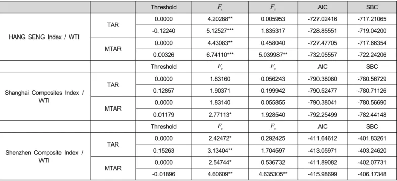
AlphaShares China Volatility Index is used as threshold in this study. The TAR/MTAR test results are presented in Tables 4. In the cases of Shanghai Composites Index and Shenzhen Composite Index, the threshold values of MTAR model are smaller than the threshold values of TAR model. Most of AIC and SBC of MTAR model are smaller than those in the TAR model. Therefore, MTAR model is better than TAR model in China and Hong Kong stock markets. Table 4 shows that most of the ^F

^c

values are significant at 1% or 5% or 10% levels in both TAR and MTAR models. Therefore, the results reject the null hypothesis ( H

⁰

^: ρ

¹

⁼ ρ

²

^{= 0} ). This represents the existence of cointegration. In the other words, the relationship is stationary in long-term between stock price indexes and spot oil price.

F

a

( H

⁰

^: ρ

¹

≠ ρ

²

) in Table 4 is used to test the symmetrical relationships between stock price indexes and oil price in the short-term. ^F

^a

of HANG SENG Index /WTI, and ^F

^a

of Shenzhen Composite Index /WTI are significant at 5% level in the MTAR models. This indicates that HANG SENG Index and WTI oil price, Shenzhen Composite Index and WTI oil price are symmetrical in the short-term. ^F

^a

of Shanghai Composites Index /WTI is not significant both in the TAR and MTAR models. This indicates that there is no symmetrical adjustment between the

residuals of Shanghai Composites Index and WTI oil price.

The results of TAR/MTAR cointegration tests show that the long-term relationships between stock price and oil price are nonlinear for HANG SENG Index, Shanghai Composites Index, and Shenzhen Composite Index, especially HANG SENG Index.

Therefore, the nonlinear threshold error correction model can be used to examine the relationships between HANG SENG Index and WTI oil price, between Shanghai Composites Index and WTI oil price,and between Shenzhen Composite Index and WTI oil price.

4.3. Threshold Error Correction Model

The asymmetric threshold error correction model (TECM) with consistent threshold estimates is used to capture the nonlinear relationships between HANG SENG Index and WTI oil price, be- tween Shanghai Composites Index and WTI oil price, and be- tween Shenzhen Composite Index and WTI oil price. Standard T test is used to study whether coefficients of STOCKi Δ and Δ WTI are statistically different from zero, and whether the co- efficients of the error-correction terms are significantly different from zero. With the appropriate lag lengths being determined by AIC, the results are presented in tables 5 and 6. Table 5 shows the results of dependent variable Δ STOCK and in- dependent variable ^{Δ WTI} . The results of dependent variable Δ WTI and independent variable STOCK Δ are shown in table 6.

Table 5 shows that the threshold ( = ASC-VIX γ ) is 39.79 for HANG SENG Index as dependent variable. Because β

3

and β

4

are not significant, WTI does not influence HANG SENG Index

<Table 4> TAR/MTAR cointegration test between Stock and WTI

Threshold F

c

F

_a

_{AIC SBC}

HANG SENG Index / WTI

TAR 0.0000 4.20288** 0.005953 -727.02416 -717.21065

-0.12240 5.12527*** 1.835317 -728.85551 -719.04200

MTAR 0.0000 4.43083** 0.458040 -727.47705 -717.66354

0.00326 6.74110*** 5.039987** -732.05557 -722.24206

Threshold F

c

F

_a

_{AIC SBC}

Shanghai Composites Index / WTI

TAR 0.0000 1.83160 0.056243 -790.38080 -780.56729

0.12857 1.90371 0.199942 -790.52477 -780.71126

MTAR 0.0000 1.83140 0.055855 -790.38041 -780.56690

0.01179 2.77113* 1.928540 -792.25499 -782.44148

Threshold F

c

F

_a

_{AIC SBC}

Shenzhen Composite Index / WTI

TAR 0.0000 2.42472* 0.292425 -411.64612 -401.83261

0.15263 3.13404** 1.704597 -413.05971 -403.24620

MTAR 0.0000 2.54744* 0.536732 -411.89082 -402.07731

-0.01896 4.60609** 4.635305** -415.98699 -406.17348

1. The critical values of F test for TAR and MTAR are from Enders and Siklos (2001).

2. F

^c

_and F

_a

denotes the cointegration test and asymmetric test, respectively.

3. ***, **, and * denote the significant levels at 1%, 5%, and 10%.

when ASC-VIX is below the threshold. α

3

is significant at 1%

level. Therefore, the lagged one period WTI oil price influences current period HANG SENG Index above the threshold. And the coefficient is negative. A negative coefficient means that WTI oil price and HANG SENG Index will move toward different direction. When HANG SENG Index rises, WTI oil price will fall.

The result of short-term causality test and long-term causality test are all significant at 1% level. This indicates that, both short-term and long-term, WTI price is able to influence HANG SENG Index. Both α

5

and β

5

are negative and significant at 1%

level. These indicate that WTI oil price and HANG SENG Index can adjust to long-term equilibrium. Table 6 shows that the threshold is 44.34 for HANG SENG Index as independent variable. No matter ASC-VIX is above or below the threshold, the lagged one and two period HANG SENG Index can influ- ence current period WTI oil price. α

1

, α

2

, β

1

and β

2

in Table 6 are all significant. And the coefficients are negative. WTI oil price and HANG SENG Index will move toward different direction. The short-term causality test and long-term causality test are all significant at 1% level. These mean, both in short-term and long-term, HANG SENG Index is able to influ- ence WTI oil price. Another α

5

and β

5

in Table 6 are negative and significant at 1% level; these indicate that WTI oil price and HANG SENG Index can adjust to long-term equilibrium.

Table 5 shows that the threshold is 36.45 for Shanghai Composites Index as dependent variable. α

3

and β

3

both are significant at 10% level. This means no matter ASC-VIX is above or below the threshold; the lagged one-period WTI oil price has influence on the current period Shanghai Composites Index. With negative coefficients means WTI oil price and Shanghai Composites Index move toward different directions.

The short-term causality test and long-term causality test are all significant at 1% level. These mean, both in the short-term and long-term, WTI oil price is able to influence Shanghai Composites Index. Both α

5

and β

5

are negative and significant at 1% level. These indicate that WTI oil price and Shanghai Composites Index could adjust to long-term equilibrium. Table 6 shows that the threshold is 45.87 for Shanghai Composites Index as independent variable. No matter ASC-VIX is above or below the threshold, the lagged one period Shanghai Composites Index can influence current period WTI oil price.

Both α

1

and β

1

in Table 6 are all significant and the coefficients are negative. WTI oil price and Shanghai Composites Index will move toward different directions. The long-term causality test is significant at 1% level. This means that, Shanghai Composites Index is able to influence WTI oil price in the long-term. Both α

5

and β

5

in Table 6 are negative and significant at 1% level.

These indicate that WTI oil price and Shanghai Composites Index can adjust to long-term equilibrium.

Table 5 shows that the threshold is 39.03 for the Shenzhen Composite Index as dependent variable. No matter ASC-VIX is above or below the threshold, the lagged one and two period WTI oil prices have no influence on the current period Shenzhen Composite Index. But the results of short-term cau-

sality test and long-term causality test are all significant at 1%

level. These mean that, both in the short-term or long-term, WTI is able to influence Shenzhen Composite Index. Both α

5

and β

5

are negative and significant at 1% level. These indicate that WTI oil price and Shenzhen Composite Index could adjust to long-term equilibrium. Table 6 shows that the threshold is 45.87 for the Shenzhen Composite Index as the independent variable.

The lagged two periods Shenzhen Composite Index can influ- ence the current WTI oil price when ASC-VIX is above the threshold. α

2

in Table 6 is significant. But the coefficient is negative. Therefore, WTI oil price and Shenzhen Composite Indexwill move toward different directions. The long-term cau- sality test is significant at 1% level. This means, in long-term, WTI oil price is able to influence Shenzhen Composite Index. α

5

and β

5

in Table 6 are negative and significant at 1% level.

These indicate that WTI oil price and Shenzhen Composite Indexcan adjust to long-term equilibrium.

The relationship between WTI and HANG SENG Index is more significant than the relationship between WTI and Shanghai Composites Index or Shenzhen Composite Index, when used investor sentiment as the thresholdvariable. The rea- sons may be that China has many natural resources and en- ergy, but Hong Kong lacks and totally dependents on imported, and there fore HANG SENG index has higher sensitivity to changes in international oil prices; it is to say when investor sentiment variable above threshold value, the degree of oil price impacting on HANG SENG index is deeper than Shanghai Composites Index or Shenzhen Composite Index. The other hand, it may be Hong Kong's economic freedom index is very high, and the account of IPO in Hong Kong Exchanges and Clearing Limited (HKEx) is the most in the world from 2009 to 2011, as a result HANG SENG Index can impact on WTI, and more significant than China.

Another, if only consider Shanghai Composites Index and Shenzhen Composite Index of China, the relationship between Shanghai Composites Index and WTI is more significant than Shenzhen Composite Index under investor sentiment as the threshold variable.

5. Conclusion

The purpose of this research is to study the nonlinear rela- tionship between stock price index and oil price, which is under the different investor sentiment in China and Hong Kong. The variables are daily closing prices, consist of Shanghai Composites Stock Index and Shenzhen Composite Stock Index of China, HANG SENG Index of Hong Kong, Spot Price of WTI crude oil, and used AlphaShares Chinese Volatility Index (ASC-VIX) as investor sentiment variable and as threshold.

The result was the relationship between stock price index

and oil price is different under the different investor sentiment,

but stock price index and oil price could adjust to long-term

equilibrium, and long-term causality test between stock price in-

<Table 5> TECM estimation – Dependent Variable: Δ STOCK

i

, Independent Variable: Δ WTI

HANG SENG Index Shanghai Composites Index Shenzhen Composite Index 1--PLUS

α 0.190530216***

(3.18848) 0.107666129*

(1.75261) 0.042834844

(0.60621) 2--PLUS

α 0.145717514***

(3.46003) 0.144247100***

(3.20667) 0.161415432***

(3.17988) 3--PLUS

α -0.163442352***

(-6.57152) -0.034229480*

(-1.66154) -0.025344006

(-1.07514) 4--PLUS

α -0.035699303

(-1.53190) -0.021343712

(-1.05713) -0.008516683

(-0.36266) 5--PLUS

α -1.264716592***

(-17.02952) -1.113516662***

(-15.36775) -0.995461383***

(-12.05529) 1--MINUS

β -0.108300510

(-1.31876) -0.170258496**

(-2.53281) -0.083628371

(-1.49997) 2--MINUS

β -0.074838963

(-1.38351) -0.086542680**

(-1.92555) -0.077318280*

(-1.90578) 3--MINUS

β -0.049385358

(-1.38744) -0.058007574*

(-1.77460) -0.045227424

(-1.31674) 4--MINUS

β -0.023948001

(-0.73563) -0.010654063

(-0.32192) -0.024095404

(-0.71331) 5--MINUS

β -0.941693603***

(-9.27748) -0.885078701***

(-10.51471) -0.889607628***

(-13.13477)

γ 39.79 36.45 39.03

Short-term Causality Test 11.97177*** 10.28273*** 10.11165***

Long-term Causality Test 15.50827*** 6.28096*** 4.56332***

AIC -767.21685 -815.15287 -584.76692

SBC -708.37188 -756.30790 -525.92195

L-BQ(12) 27.196*** 10.893 8.830

L-BQ2(12) 780.094*** 343.637*** 333.485

1. ( ): T-Stat

2. ***, **, and * denote the significant levels at 1%, 5%, and 10%

<Table 6> TECM estimation – Dependent Variable: WTI, Independent Variable: STOCKi Δ Δ

HANG SENG Index Shanghai Composites Index Shenzhen Composite Index 1--PLUS

α -0.385358137***

(-6.73308) -0.354982018***

(-5.12961) -0.386756239***

(-5.58742) 2--PLUS

α -0.108560627**

(-1.97813) -0.010674238

(-0.15001) -0.106666221

(-1.49643) 3--PLUS

α 0.243872486***

(4.03611) 0.226807251***

(4.00064) 0.198605278***

(3.51846) 4--PLUS

α 0.191686680***

(4.35017) 0.183614885***

(4.47064) 0.172016884***

(4.21079) 5--PLUS

α -1.203897327***

(-15.92373) -1.167427228***

(-16.60088) -1.156510638***

(-16.63197) 1--MINUS

β -0.275436049***

(-4.15116) -0.085516984*

(-1.74465) -0.065890160

(-1.59517) 2--MINUS

β -0.172898673**

(-2.83118) -0.028378409

(-0.59186) -0.021926502

(-0.53640) 3--MINUS

β 0.024198074

(0.30630) 0.009406289

(0.13126) 0.010679126

(0.15048) 4--MINUS

β 0.036923024

(0.68766) 0.040096273

(0.80996) 0.042073383

(0.85514) 5--MINUS

β -1.037924925***

(-10.72762) -1.018092807***

(-11.75747) -1.015853896***

(-11.86213)

γ 44.34 45.87 45.87

Short-term Causality Test 3.91299** 0.02250 2.23930

Long-term Causality Test 11.56455*** 6.42951*** 6.27499***

AIC 42.35075 -8.33585 -18.26606

SBC 101.19571 50.50911 40.57891

L-BQ(12) 29.135*** 22.390** 23.235**

L-BQ2(12) 434.522*** 443.190*** 489.480***

1. ( ): T-Stat

2. ***, **, and * denote the significant levels at 1%, 5%, and 10%

dex and oil price were all significant. When used investor senti- ment as the threshold variable, the relationship between WTI and HANG SENG Index is more significant than the relationship between WTI and Shanghai Composites Index or Shenzhen Composite Index, and Shenzhen Composite Index is weakest.

The empirical results of the paper offer four major findings.

First, there is evidence that the correlation between the stock and oil markets is not constant but time-varying. It tends to in- crease with the volatility in the market. Second, the daily vola- tility in each market is very persistent. That is, it varies over time in a predictable manner, conditioned on the past volatilities.

Third, there is bidirectional dependence in volatility between the two markets. Innovations that hit either market can affect the volatility in the other market. In other words, conditioned on the persistence and the past volatility in their markets, the past vol- atility of the stock (oil) market also has predictive power over the future volatility of the oil (stock) market.

The different of relationship between oil price and stock price index under investor sentiment as the threshold variable, may be about one self’s resources and energy, but other reasons, example: economic freedom, the account of IPO , perhaps give … deep influences.

References

Driesprong, G., Jacobsen, B., & Maat, B. (2008). Striking oil:

Another puzzle? Journal of Financial Economics, 89, 307 327.

–

El-Sharif, I., Brown, D., Burton, B., Nixon, B., &Russell, A.

(2005). Evidence on the nature and extent of the rela- tionship between oil prices and equity values in the U.K.

Energy Economics, 27, 819 830. –

Gisser, M., & Goodwin, T.H. (1986). Crude oil and the macro- economy: tests of some popular notions. Journal of Money, Credit, and Banking, 18, 95 103. –

Jones, C., & Kaul, G. (1996). Oil and the stock markets.

Journal of Finance, 51, 463 491. –

Jones, D.W., Leiby, P.N., & Paik, I.K. (2004). Oil price shocks and the macroeconomy: what has been learned since 1996. Energy Journal, 25, 1 32. –

Kanas, Angelos (2012). Modelling the risk return relation for the – S&P 100: The role of VIX. Economic Modeling, 29, 795-809.

Merton, R.C. (1973). An intertemporal capital asset pricing model. Econometrica, 41, 867 887. –

Minh Vo. (2011). Oil and stock market volatility: A multivariate stochastic volatility perspective. Energy Economics, 33, 956 965 –

Papapetrou, E. (2001). Oil price shocks, stock market, economic activity and employment in Greece. Energy Economics, 22, 511 532. –

Park, J., Ronald A., & Ratti, R.A. (2008). Oil price shocks and stock markets in the U.S. and 13 European countries.

Energy Economics, 30, 2587 2608. –

Rotemberg, J.J., & Woodford, M. (1996). Imperfect competition and the effects of energy price increases on economic activity. Journal of Money, Credit and Banking, 28, 549–

577.

Sadorsky, P. (2001). Risk factors in stock returns of Canadian oil and gas companies. Energy Economics, 23, 17 28. – Sari, R., Soytas, U. & Hacihasanoglu, E. (2011). Do global risk

perceptions influence world oil prices? Energy Economics, 33, 515 524. –

Whaley, R.E. (2000). The investor fear gauge. Journal of

Portfolio Management, 26, 12 17. –