Print ISSN: 2288-4637 / Online ISSN 2288-4645 doi:10.13106/jafeb.2021.vol8.no2.0015
Day-of-the-Week Effect of Exchange Rate in Developing Countries
Cep Jandi ANWAR1, Nicholas OKOT2, Indra SUHENDRA3
Received: November 05, 2020 Revised: December 30, 2020 Accepted: January 08, 2021
Abstract
This study investigates the presence of the day-of-the-week anomaly in exchange rate for 30 developing countries with free floating exchange rate regimes using daily data from January 2, 2011 to December 31, 2019. First, we apply the GARCH panel to estimate the intraday effect for all the sampled countries. Second, we run poolability test to check whether the coefficients of the GARCH panel are the same for all countries sampled. The result of poolability test rejects the homogeneity assumption. This implies that our sample countries contain heterogeneity. Third, we apply mean-group estimation by averaging the coefficients for all individual GARCH estimations. Fourth, we divided our sample of developing countries into three groups based on capital restriction index for the reason that the effect of monetary policy on the exchange rate depends on the degree of capital account liberalization. The empirical evidence for the return equation suggests that Mondays are connected with lower volatility whereas Thursdays experiences higher return compared to Tuesdays. The lowest estimated coefficient for full sample, group 1 and group 2, is Friday, but for group 2 is Thursday. We find similar result for the volatility equations, which show that Monday returns are lower compared to Tuesday.
Keywords: Exchange Rate, Day of the Week Effect, GARCH, Heterogeneity, Poolability Test JEL Classification Code: C58, G14, G15
studies where the reported evidence appears to contradict the EMH assumption, stock index returns appear to be related to certain fundamental characteristics of the firm (e.g., stock- value vs share-growth, multiple EPS, etc.).
Kristjanpoller Rodrıguez (2009) states that the anomaly in the intraday effect consists of regular observations of stock market returns and volatility that differ significantly from the average on a particular day of the week. The literature has largely focused on the day- of-the-week effects on stock market returns in developed and emerging market economies. In developing countries, where stock markets are not well developed, the foreign exchange market is considered the most efficient in terms of information and the transmission of shocks where the floating exchange rate regime is the policy framework (Andriyani et al., 2020).
In the stock market for instance, the main reason there is an intraday effect is news. The behavioral financial literature proposes that companies release bad news that is likely to affect equity prices over the weekend, but releases good news sooner. Thus, Monday’s returns tend to be negative.
Zhang et al. (2017) also note that companies usually report bad news near the end of the week, and especially after the close of trading on Friday. This bad news affects the return of the next trading day, which is usually Monday.
1 First Author and Corresponding Author. Department of Economics, Faculty of Economics and Business, Universitas Sultan Ageng Tirtayasa, Banten, Indonesia [Postal Address: Jl. Raya Jkt Km 4 Jl.
Pakupatan, Panancangan, Kec. Cipocok Jaya, Kota Serang, Banten 42124, Indonesia] Email: [email protected]
2 Statistics Department, Bank of Uganda, Uganda.
Email: [email protected]
3 Department of Economics, Faculty of Economics and Business, Universitas Sultan Ageng Tirtayasa, Banten, Indonesia.
Email: [email protected]
© Copyright: The Author(s)
This is an Open Access article distributed under the terms of the Creative Commons Attribution Non-Commercial License (https://creativecommons.org/licenses/by-nc/4.0/) which permits unrestricted non-commercial use, distribution, and reproduction in any medium, provided the original work is properly cited.
1. Introduction
The day-of-the-week implies that the yields can be predicted based on the day trading taking place on the financial markets. Empirical research by Gayaker et al.
(2020) proves in financial markets that returns on Friday are higher than Monday. According to the Efficient Market Hypothesis (EMH), market participants cannot obtain abnormal yields based on the public information they have.
In this situation, the expected yields in an efficient market on each working day should be about the same. In several
There are several features of the existing literature that motivate this paper. First, there is inconclusive empirical evidence on the existence of the day-of-the-week anomalies of exchange rate returns. For example, Ranaldo (2009) states that exchange rate tend to appreciate during foreign trading hours while Breedon and Ranaldo (2013) find the opposite result.
Second, the existing study only estimates the day-of-the- week pattern for individual countries. Hence, there exists a gap of recent study of the day-of-the-week effects on foreign exchange trading for developing countries. Furthermore, there is a lack of evidence regarding the day-of-the-week patterns in exchange rate markets for developing economies to suggest whether this high frequency calendar anomaly occurs with a similar or random pattern. This paper is motivated by the desire to fill this research gap in the empirical evidence of intraday effects in the exchange rate markets for a sample of developing countries operating under the floating exchange rate regime.
This study adds to the literature in many ways. First, we use an information-rich Generalized Autoregressive Conditional Heteroskedasticity (GARCH) panel approach to investigate an intraday effect. Simultaneously, this methodology is enhanced by previous studies of intraday pattern by controlling for heterogeneity among developing countries. In other words, it is possible to estimate an intraday assuming the results are the same for all sample countries. To the best of our knowledge, no previous study investigated the effects of trading days on currency market in developing countries with floating exchange rate regimes using the GARCH panel. Second, our approach makes it possible to find the intraday effect in both conditional mean and conditional variant equations for all countries sample.
However, removing the intra effect from both equations can lead to false conclusions about the cross-sectional intensity of dependence. Hence, by applying a GARCH panel model provides more accurate cross-country correlations incorporate with the day-of-the-week effect.
The remainder of this paper is structured as follows.
Section 2 discusses the literature review on the day of the week effect of exchange rate, while section 3 describes the data set used for the empirical analysis and discusses the methodological approach. Section 4 presents the results of GARCH regression and discussion. Section 5 is the conclusion.
2. Literature Review
The empirical literature has largely relied on time-series econometric methods to examine the within country effects, but there has been a gradual increase in the application of panel approach to evaluate the cross-countries effects. The intraday effect on exchange rates has been one of the most interesting areas of research of the past decade given the increased
globalization of finance and move toward flexible exchange rate regime. Santillán Salgado et al. (2019) investigated the intraday effect of exchange rates based on data sets for six South American countries, namely, Argentina, Brazil, Chile, Colombia, Mexico, and Peru using daily data for the period January 3, 2003, to October 23, 2018. They applied the TARCH estimate to investigate this anomaly because it estimated the conditional variance as a stationary trend.
They concluded that the volatility of shocks remained in their sample countries, except Chile. In addition, they found the presence of intraday effect that existed throughout the week in Argentina and Peru; Monday, Tuesday and Friday effects were detected for Mexico; Wednesday and Thursday effects were present for Chile; however, they found no evidence of day-of-the-week effect for Brazil and Colombia.
Similarly, Yamori and Kurihara (2004) examined intraday effect of 29 currencies in the New York market using daily data from 1980s and 1990s. They find that market anomaly exists in the 1980s, but disappeared in the 1990s for European exchange rate. Cohay (1995) investigated the existence of day-of-the-week effects in six currencies, including the Canadian dollar, British pound, Japanese yen, Deutsch mark, Swiss franc and French franc from January 1973 to December, 1992, using GARCH estimation approach to account for variations time in a variant of the exchange rate series. Their findings revel that Wednesday’s return was the highest for all currency samples.
Ke, Chiang, and Lias (2007) employed the stochastic- dominance method with and without risk-free assets to test whether the intraday effect can affect the pattern of exchange rate return on the Taiwanese exchange rate market. They use daily data from January 1992 to April 2006 for foreign currencies of US dollar, Australia dollar, UK pound, Canada dollar, Euro, Swiss franc, Japan yen and Hong Kong dollar against the new Taiwan dollar. They divided their period sample into three sub-periods based on Taiwan currency market trading regime. They find that in the first sub-period (1992-1997) and third sub-period (2001-2006), participants can get higher returns in the Taiwan exchange rate on Monday, Tuesday and Wednesday for all currencies against new Taiwan dollar.
Berument et al. (2007) evaluated the presence of intraday anomaly on the Turkish currency against United States dollar. Their finding shows that Thursday is associated with higher currency depreciation, and Monday related to lower depreciation, comparing the two with Wednesday. Moreover, they reported that Monday and Tuesday are related to higher volatility than Wednesday. Romero-Meza et al. (2010) used a new approach to detect subtle periodicity in the Chilean peso currency market. They offer explanations for the discovered microstructural behavior, including the intraday effect, in which they shows that the market follows a different pattern of behavior trader.
Khademalomoom and Narayan (2019) conducted a study of the intraday effect of six world currencies including the British Pound, Australian Dollar, Japanese Yen, Canadian Dollar, Swiss Franc and Euro against the United States Dollar over the period 2004 to 2014.
They found three new day-of-the-week effects that are different from other studies, namely, the post-local market opening effect, the main market activity effect, and the market overlap timing effect. They also point out that the currency behavior caused by these the day-of-the- week effects has implications for investors. Singh (2019) analyzed the intraday effects in the volatility exchange rate for the data of 10 pairs currencies. His study performed the univariate GARCH for each currency pair. His main result is the Monday effect on the fear sentiment for all sample countries, which shows a high positive return of substantial value, and the Friday effect represents a negative return.
3. Data and Methodology 3.1. Data
The exchange rate data for the analysis were obtained from Bloomberg. We select 30 developing countries (Afghanistan, Albania, Brazil, Chile, Colombia, Gambia, Georgia, Ghana, Guatemala, India, Indonesia, Kenya, Madagascar, Mauritius, Mexico, Moldova, Mongolia, Peru, Philippines, Poland, Romania, Serbia, Seychelles, South Africa, Tanzania, Thailand, Turkey, Uganda and Uruguay, Zambia) that apply floating exchange rate regime for the reason that exchange rate is based on market equilibrium.
This paper uses daily foreign exchange data for each country covering the period from 2nd January 2011 to 31st December 2019. The reason we selected the data after the global financial crisis is to avoid outlier in the currency market for the sample countries.
3.2. Econometrics Methodology
We employ a method similar to that of Zhang et al.
(2017) and Nguyen et al. (2020) to investigate the effect of day of the week on foreign currencies among a sample of developing countries. In particular, Zhang et al. (2017) used regression with weekday dummies to study intraday effects on the stock market, and determined variance as a GARCH (1,1) process to describe dynamic volatility.
We apply GARCH (1,1) model because GARCH (1,1) performed best in modeling volatility of stock returns or exchange rate volatility. It is relatively simple to setup and calibrate because it relies on past observations. The compact representation of the GARCH (1,1) model are specified as follows:
( )
51φ , ε
= ∑ +
Rt i= i i tD t (1) and
2 2 2
1 1
δt = +w αåt− +βδt− (2) where daily return (Rt) is the raw foreign exchange rate, Di,t (i = 1 , 2 , . . . , 5) are dummy variables such that Di,t = 1 if day t is the i the intraday and Di,t = 0 otherwise. φi (i
= 1,2,…, 5) are coefficients and εt is the error term. δt2 is s the conditional variance of is the constant term, α and β are coefficients, δt2−1 is the lag term of δt2. To determine whether φi is significantly different from zero or not, we observe the t value after estimation.
This paper uses a standard regression model approach of the intraday effects to investigate the anomaly effect on exchange rates. The exchange rate for each country (i) is calculated as the percentage change in the daily local exchange rate against the US dollar over the same period from the previous day.
, , 1
,
, 1
− 100
−
= i t− i t ×
i t
i t
S S
R S (3)
where Si,t is the exchange rate level of country i at time t.
In this study we run two models to investigate the day of the week effect. Our first model is return model, which consists of the following two equations:
0
, 1
α α α α α
α − λ
=
= + + + +
+∑ + +å
it M it T it W it F it
n
i i t it it
I i
R M T W F
R h
(6)
2 2 2
, 1− , 1−
= + å +
it c a i t b i t
h V V V h (7)
where Ri,t represents returns on foreign exchange for each country, Mi,t, Ti,t, Wi,t, and Fi,t are the dummy variables for Monday, Tuesday, Wednesday, and Friday at time t, and n is the lag order. λ is a measure of the risk premium in the foreign exchange market. If λ is positive, then risk-averse agents must be compensated to accept higher risk. Here, we take into account the possibility that the lagged values of the squared residuals and the conditional variances might be too restrictive.
Our second model is return and volatility exchange rate model, which specified as follows:
0
, 1
α α α α α
α − λ
=
= + + + +
+∑ + +å
it M it T it W it F it
n
i i t it it
I i
R M T W F
R h
(8)
2
2 2
, 1 , 1
it c M it T it W it
F it a i t b i t
h V V M V T V W V F V ε − V h −
= + + +
+ + + (9)
4. Empirical Results and Discussion 4.1. Descriptive Statistics
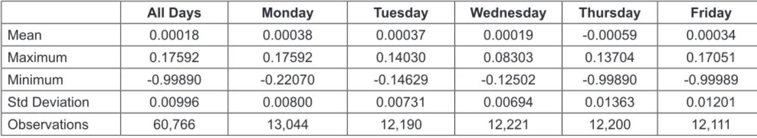
Table 1 shows descriptive statistics for daily returns for all sample countries. Overall, the average daily returns are positive at 0.00018; meanwhile, on a daily basis, the largest numbers are Monday (0.00038), Tuesday (0.00037), Wednesday (0.00019), Thursday (-0.00059) and Friday (0.00034). So, we can conclude that the largest return is on Monday, but the lowest return is on Thursday. Meanwhile, the average for Wednesday is almost the same as the average for the full samples. In terms of maximum value, the largest is for Monday (0.017592), while the smallest is Wednesday (0.08303). The minimum value is in the range -0.125 to -1. Meanwhile, the standard deviation ranges from 0.007 to 0.0136. This suggests that there are lower volatility on Wednesday and Tuesdays. Overall, the summary statistics indicate those exchange rates are more volatile on Thursdays for these developing countries.
4.2. Full Sample Countries
The residual squared partial autocorrelation coefficient of the fixed-effects panel model is calculated as in Arneric et al. (2018). The results in Table 2 show that all partial autocorrelation coefficients to lag 5 are statistically significant at the 1% level. The amount of delay included in the test corresponds to the number of trading days in a week. This findings show that the existence of time-varying variance, that is, conditional heteroscedasticity. Therefore, it is necessary to introduce a conditional variant equation that follows the GARCH (1,1) process.
The results in Table 2 supports the presence of ARCH effects in the model. Thus, we need to perform a combination of panel data and GARCH methodology to examine the intraday effect.
Table 3 reports the day-of-the-week effects on return equation of exchange rate for a panel of 30 developing countries. We exclude Tuesday’s dummy variable from the equation to avoid the dummy variable trap. We chose not to include Tuesday because the average Tuesday is similar to Monday. Therefore, the estimated coefficient of Monday, Wednesday, Thursday and Friday can be compared with the return on Tuesday. The estimated coefficients of the Monday’s dummy variable is -0.001116, Wednesday’s dummy variable is -0.001264, Thursday’s dummy variable is -0.004704 and Friday’s dummy variable is -0.001496 and they are statistically significant at 1%. So that we can conclude that there is a market anomaly where Monday’s return is significantly smaller than Thursday’s return.
4.3. Poolability Test
The preceding results assume that the coefficients day of the week effect are homogeneous for all countries and ignore the possibility of heterogeneity in the sample.
Therefore, this study tests the pooling assumption in the model to check whether or not the coefficients for all variables are poolable. We run a non-standard poolability test to verify whether or not the model is poolable by using a dummy variable approach. To do so, we will compare two models, namely the restricted and unrestricted models. The unrestricted model is the general model in Equation (6), while this test uses a dummy variable approach where D=0, except for country i where D=1 for the restricted model.
This model multiplies the dummy variable for each of the dependent variables. Consequently, the slope is allowed to vary because both conditions (0 and 1) associated with the dummy variable.
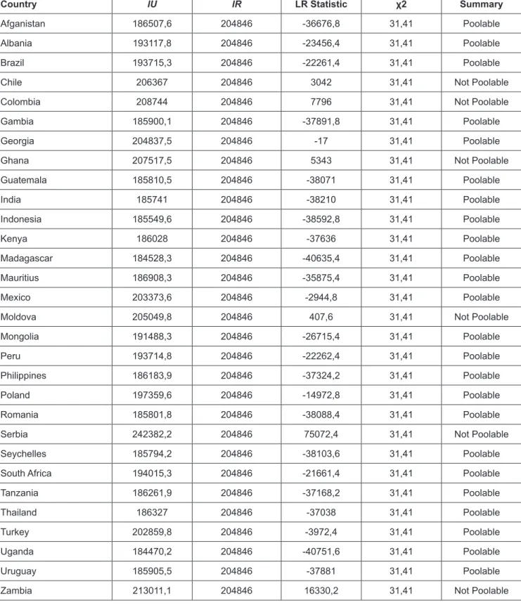
Table 4 shows the result of the poolability test using the dummy variable approach. From 30 countries in the sample, the result shows that 24 countries are poolable, while six countries are not. This result implies that the homogeneity assumption for full sample does not hold. This signifies that the coefficients are not the same for every country. Thus, the result concludes the existence of heterogeneity in the model and that the result in Table 3 is biased.
4.4. Mean Group GARCH Full Sample and GARCH Sub Sample
Given that our result using panel GARCH is not poolable means that the coefficients in the model are not the same for all countries. To solve this problem, we apply the idea of a mean-group estimation by running GARCH estimation for individual country and averaging the coefficients.
According to Davis and Zlate (2019), the effect of monetary policy on the exchange rate depends on the degree of capital account liberalization for each country.
On that basis, we also divide the sample into three sub- groups based on capital restriction – low, moderate, and high restrictions. Group 1, which includes countries that have low capital restrictions, consists of Georgia, Ghana, Guatemala, Kenya, Mauritius, Peru, Romania, Uganda, Uruguay and Zambia. Group 2, namely, countries with moderate capital restrictions, includes Brazil, Chile, Colombia, Indonesia, Mexico, Moldova, Poland, South Africa, Thailand, Turkey.
Meanwhile, Group 3 consists of countries with high capital restrictions, namely, Afghanistan, Albania, Gambia, India, Madagascar, Mongolia, Philippines, Serbia, Seychelles and Tanzania.
Table 1: Descriptive Statistics
All Days Monday Tuesday Wednesday Thursday Friday
Mean 0.00018 0.00038 0.00037 0.00019 -0.00059 0.00034
Maximum 0.17592 0.17592 0.14030 0.08303 0.13704 0.17051
Minimum -0.99890 -0.22070 -0.14629 -0.12502 -0.99890 -0.99989
Std Deviation 0.00996 0.00800 0.00731 0.00694 0.01363 0.01201
Observations 60,766 13,044 12,190 12,221 12,200 12,111
Table 2: Partial Autocorrelation Coefficients Test
Lag PAC p-value Q p-value
11 0.057 0.000 194.24 0.000
22 -0.019 0.000 217.35 0.000
33 -0.009 0.000 225.43 0.000
44 -0.013 0.000 237.58 0.000
55 0.021 0.000 261.82 0.000
Table 3: Intraday Effect in Return Equation
Full Sample Return Equation
Constant -0.000768**
(0.000145)
Monday -0.001116***
(0.000191)
Wednesday -0.001264***
(0.000205)
Thursday -0.004707***
(0.000074)
Friday -0.001496***
(0.000199)
Returnt-1 -0.164126***
(0.000561)
Risk 0.035603***
(0,002939) Volatility
Va 0.223510***
(0.065312)
Vb 0.999967***
(0.00000005)
Vc 0.0000328***
(0.000000005) Notes:
1. The dependent variable is Return.
2. Standard errors are in parentheses.
3. The symbols *, **, *** denote statistical significance at the 10%, 5% and 1% level.
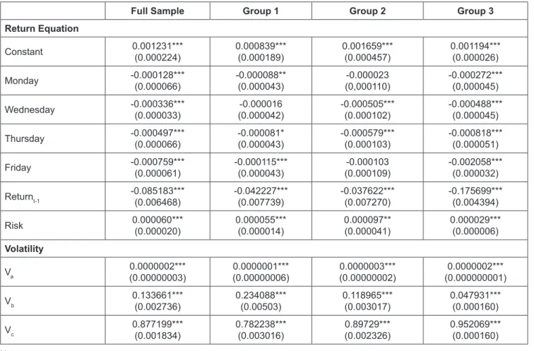
Table 5 reveals the GARCH estimation for all countries sample using mean group estimation and three sub-groups.
The results in the table reveal the day-of-the-week effect from the foreign exchange return equations 6 and 7. The coefficients for Monday’s dummy are -0.000128, -0.000088, -0.000023 and -0.000272 for the full sample, groups 1, 2 and 3 and it is significant at 1% level for full sample and group 3, significant at 5% level for group 1 , while for group 2 it is not significant. These findings indicate that the return on Monday is lower than Tuesday. This finding supports previous research such as Santillán Salgado et al. (2019), Singh (2019) and Khademalomoom and Narayan (2019), which concluded that there is always a depreciation of currencies in developing countries on Monday. The lowest estimated coefficient for full sample, group 1 and group 2, is Friday, but for group 2 is Thursday. This finding contradicts Zhang et al. (2017), Chiah and Zhong (2019), Birru (2018), and Romero-Meza et al. (2010), which state that the end of the weekday provides positive foreign exchange returns to traders. Our results show that the exchange rate return every day is negative, this reflects that if we compare the return each day is lower than Tuesday or in other words that Tuesday always gives the highest return for the full sample and the three subgroups.
The regression coefficient of the conditional standard deviation of the exchange rate return (risk) is positive and significant at 1% level for all groups. This shows that market players want to get positive yields because they have risky assets with higher returns (Lee & Brahmasrene, 2019). The coefficient for the constant term for the conditional variance equation (Va) is positive and statistically significant at the 1% level for the entire group sample. This suggests that a positive unexpected change in the depreciation equation leads to more changes in the conditional variant than a negative unexpected change. The coefficient for lagged value of the squared residual term (Vb) is positive and significant at 1%
level. The regression results show that the largest is for group 1 and the smallest is for group 3. Meanwhile, the lagged value of the conditional variance (V(c)) is positive and significant at level 1%, with the highest value for group 3 and lowest for group 1. These results show that the conditional variance is positive which means that the conditional variance for the whole group is non-explosiveness (Berument et al., 2007).
Table 4: Poolability Test
Country lU lR LR Statistic χ2 Summary
Afganistan 186507,6 204846 -36676,8 31,41 Poolable
Albania 193117,8 204846 -23456,4 31,41 Poolable
Brazil 193715,3 204846 -22261,4 31,41 Poolable
Chile 206367 204846 3042 31,41 Not Poolable
Colombia 208744 204846 7796 31,41 Not Poolable
Gambia 185900,1 204846 -37891,8 31,41 Poolable
Georgia 204837,5 204846 -17 31,41 Poolable
Ghana 207517,5 204846 5343 31,41 Not Poolable
Guatemala 185810,5 204846 -38071 31,41 Poolable
India 185741 204846 -38210 31,41 Poolable
Indonesia 185549,6 204846 -38592,8 31,41 Poolable
Kenya 186028 204846 -37636 31,41 Poolable
Madagascar 184528,3 204846 -40635,4 31,41 Poolable
Mauritius 186908,3 204846 -35875,4 31,41 Poolable
Mexico 203373,6 204846 -2944,8 31,41 Poolable
Moldova 205049,8 204846 407,6 31,41 Not Poolable
Mongolia 191488,3 204846 -26715,4 31,41 Poolable
Peru 193714,8 204846 -22262,4 31,41 Poolable
Philippines 186183,9 204846 -37324,2 31,41 Poolable
Poland 197359,6 204846 -14972,8 31,41 Poolable
Romania 185801,8 204846 -38088,4 31,41 Poolable
Serbia 242382,2 204846 75072,4 31,41 Not Poolable
Seychelles 185794,2 204846 -38103,6 31,41 Poolable
South Africa 194015,3 204846 -21661,4 31,41 Poolable
Tanzania 186261,9 204846 -37168,2 31,41 Poolable
Thailand 186327 204846 -37038 31,41 Poolable
Turkey 202859,8 204846 -3972,4 31,41 Poolable
Uganda 184470,2 204846 -40751,6 31,41 Poolable
Uruguay 185905,5 204846 -37881 31,41 Poolable
Zambia 213011,1 204846 16330,2 31,41 Not Poolable
Table 5: Intraday Effect in Return Equation
Full Sample Group 1 Group 2 Group 3
Return Equation
Constant 0.001231***
(0.000224) 0.000839***
(0.000189) 0.001659***
(0.000457) 0.001194***
(0.000026)
Monday -0.000128***
(0.000066) -0.000088**
(0.000043) -0.000023
(0,000110) -0.000272***
(0,000045)
Wednesday -0.000336***
(0.000033) -0.000016
(0.000042) -0.000505***
(0.000102) -0.000488***
(0.000045)
Thursday -0.000497***
(0.000066) -0.000081*
(0.000043) -0.000579***
(0.000103) -0.000818***
(0.000051)
Friday -0.000759***
(0.000061) -0.000115***
(0.000043) -0.000103
(0.000109) -0.002058***
(0.000032)
Returnt-1 -0.085183***
(0.006468) -0.042227***
(0.007739) -0.037622***
(0.007270) -0.175699***
(0.004394)
Risk 0.000060***
(0.000020) 0.000055***
(0.000014) 0.000097**
(0.000041) 0.000029***
(0.000006) Volatility
Va 0.0000002***
(0.00000003) 0.0000001***
(0.00000006) 0.0000003***
(0.00000002) 0.0000002***
(0.000000001)
Vb 0.133661***
(0.002736) 0.234088***
(0.00503) 0.118965***
(0.003017) 0.047931***
(0.000160)
Vc 0.877199***
(0.001834) 0.782238***
(0.003016) 0.89729***
(0.002326) 0.952069***
(0.000160) Notes:
1. The dependent variable is Return.
2. Standard errors are in parentheses.
3. The symbols *, **, *** denote statistical significance at the 10%, 5% and 1% level.
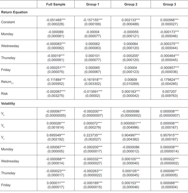
Table 6 shows the results of the regression for equations 8 and 9. In this equation, we add four new days (Monday, Wednesday, Thursday and Friday) in the volatility equation.
For the return equation, we find evidence that the results of the day-of-the-week effect are similar to the previous results in Table 5. Coefficient regression for dummy Monday for full sample (-0.000089), group 1 (-0.0004), group 2 (-0.000055) and group 3 (-0.00173), although only group 3 has significant effect at 1% level. The results show that Monday returns are lower compared to Tuesday. For the full sample and group 3, the regression estimation results show that the return on Wednesday, Thursday and Friday is statistically significantly lower than the return on Tuesday, with the lowest coefficient being Friday. For group 1, the returns for Wednesday, Thursday and Friday are higher than Tuesday although not significant, with the highest coefficient for Wednesday.
Whereas for group 2, the return on Wednesday and Friday was lower than Tuesday, but the return on Thursday was higher than that on Tuesday. The regression coefficient of the conditional standard deviation of the return equation (risk) is positive and significant for group 2 (0.000183), group 3 (0.07207), but significant negative for the full sample (-0.002067) and group 1 (-0.013591).
Next, we will see the results for the conditional variance equation. The highest volatility for full sample, group 1 and group 2 with coefficients 0.000011, -0.000189 and 0.000153 occurred on Friday. Whereas for group 3, the highest volatility occurred on Thursday with a coefficient of 0.000090. All these results are significant at the 1% level. The lowest volatility occurs on Wednesday for the full sample (-0.000068) and group 1 (-0.000332). Meanwhile, group 2 (-0.000086) and group 3 (0.000008) occurred on Monday for the smallest volatility.
Table 6: Intraday Effect in Return and Volatility Equations
Full Sample Group 1 Group 2 Group 3
Return Equation
Constant -0.051485***
(0.000228) -0.157155***
(0.000169) 0.002133***
(0.000488) 0.000566***
(0.000027)
Monday -0.000089
(0,000081) -0.00004
(0,000077) -0.000055
(0,000121) -0.000173***
(0,000046)
Wednesday -0.000083***
(0,000082) 0.000062
(0,000083) 0.000064
(0,000120) -0.000375***
(0,000044)
Thursday -0.00019***
(0,000081) 0.000101
(0,000077) -0.000205*
(0,000120) -0.000464***
(0,000045)
Friday -0.000251***
(0,000075) 0.000065
(0,000067) 0.00004
(0,000123) -0.000857***
(0,000036)
Returnt-1 -0.111884***
(0,005952) -0.161918***
(0,003302) 0.00609
(0,010269) -0.179824***
(0,004285)
Risk -0.002067***
(0,003275) -0.013591***
(0,00002) 0.000183***
(0,000042) 0.007207
(0,009763) Volatility
Va -0.000067***
(0,00000005) -0.000200***
(0,00000007) -0.0000086
(0,00000002) 0.000008***
(0,00000007)
Vb 0.000026***
(0,001814) 0.000072***
(0,000279) 0.0000001***
(0,004996) 0.000006***
(0,000167)
Vc 0.695549***
(0,002192) 0.223735***
(0,002027) 0.904997***
(0,004382) 0.957915***
(0,000167)
Monday -0.000067***
(0,000005) -0.000200***
(0,0000017) -0.0000086
(0,000012) 0.000008***
(0,0000014)
Wednesday -0.000068***
(0,000014) -0.000332***
(0,0000027) 0.000105***
(0,000040) 0.000022***
(0,0000002)
Thursday -0.000023***
(0,000017) -0.000263***
(0,0000022) 0.000105**
(0,000045) 0.000090***
(0,000005)
Friday 0.000011***
(0,000017) -0.000189***
(0,0000015) 0.000153***
(0,000046) 0.000068***
(0,000004) Notes:
1. The dependent variable is Return.
2. Standard errors are in parentheses.
3. The symbols *, **, *** denote statistical significance at the 10%, 5% and 1% level.
5. Conclusion
This study investigated the existence of intraday effect and examined the pattern of exchange rate volatility in 30 developing countries over the period January 2, 2011 to December 31, 2019. We use individual country exchange rate against the US dollars. Using panel GARCH estimation the results reveal that there is evidence of Monday effect on exchange rate in these developing countries, but there is no higher volatility on Thursdays. The poolability test rejects the homogeneity assumptions, which indicate differences between countries. Third, we apply mean- group estimation by averaging the coefficients for all individual GARCH estimation. Fourth, we divided our sample countries into three sub-groups based on capital restriction index.
The results of our empirical study reveal that the day- of-the-week pattern exists both in return and volatility equations. This study finds that for all groups the return of Monday, Wednesday, Thursday and Friday compared to Tuesday is negative for all groups. This result implies that Tuesday is the highest return in the week. Another finding of this study is the highest volatility for full sample, group 1 and group 2 is Friday, and for group 3 is Thursday.
References
Andriyani,K., Marwa, T., Adnan, N., & Muizzuddin, M. (2020).
The Determinants of Foreign Exchange Reserves: Evidence from Indonesia. Journal of Asian Finance, Economics and Business, 7(11), 629–636. https://doi.org/10.13106/jafeb.2020.
vol7.no11.629
Arnerić, J., & Perić, B. Š. (2018). Panel Garch model with cross- sectional dependence between CEE emerging markets in trading day effects analysis. Romanian Journal of Economic Forecasting, 21(4), 71.
Berument, H., Coskun, M. N., & Sahin, A. (2007). Day of the week effect on foreign exchange market volatility: Evidence from Turkey. Research in International Business and Finance, 21(1), 87–97.
Birru, J. (2018). Day of the week and the cross-section of returns.
Journal of Financial Economics, 130(1), 182–214.
Breedon, F., & Ranaldo, A. (2013). Intraday patterns in FX returns and order flow. Journal of Money, Credit and Banking, 45(5), 953–965.
Chiah, M., & Zhong, A. (2019). Day-of-the-week effect in anomaly returns: International evidence. Economics Letters, 182, 90-92.
Corhay, A., Fatemi, A. M., & Tourani-Rad, A. (1995). On the presence of a day-of-the-week effect in the foreign exchange market. Managerial Finance, 21(8), 32–43.
Davis, J. S., & Zlate, A. (2019). Monetary policy divergence and net capital flows: Accounting for endogenous policy responses.
Journal of International Money and Finance, 94, 15–31.
Gayaker, S., Yalcin, Y., & Berument, M. H. (2020). The day of the week effect and interest rates. Borsa Istanbul Review, 20(1), 55–63.
Ke, M. C., Chiang, Y. C., & Liao, T. L. (2007). Day-of-the-week effect in the Taiwan foreign exchange market. Journal of Banking & Finance, 31(9), 2847–2865.
Khademalomoom, S., & Narayan, P. K. (2019). Intraday effects of the currency market. Journal of International Financial Markets, Institutions and Money, 58, 65–77.
Kristjanpoller Rodriguez, W. (2009). An Analysis of the Day-of- the-Week Effect in Latin American Stock Markets. Lecturas de Economía, (71), 189–207.
Lee, J. W., & Brahmasrene, T. (2019). Long-run and Short-run Causality from Exchange Rates to the Korea Composite Stock Price Index. Journal of Asian Finance, Economics and Business, 6(2), 257–267. https://doi.org/10.13106/jafeb.2019.
vol6.no2.257
Nguyen, T. N., Nguyen, D. T., & Nguyen, V. N. (2020). The impacts of oil price and exchange rate on Vietnamese stock market.
Journal of Asian Finance, Economics and Business, 7(8), 143–
150. https://doi.org/10.13106/jafeb.2020.vol7.no8.143
Ranaldo, A. (2009). Segmentation and time-of-day patterns in foreign exchange markets. Journal of Banking & Finance, 33(12), 2199–2206.
Romero-Meza, R., Bonilla, C. A., Hinich, M. J., & Borquez, R. I. C.
A. R. D. O. (2010). Intraday patterns in exchange rate of return of the Chilean Peso: New evidence for day-of-the-week effect.
Macroeconomic Dynamics, 14(S1), 42–58.
Santillán Salgado, R. J., Fonseca Ramírez, A., & Romero, L. N.
(2019). The “day-of-the-week” effects in the exchange rate of Latin American currencies. Revista Mexicana De Economía Y Finanzas, 14(SPE), 485–507.
Singh, V. K. (2019). Day-of-the-week effect of major currency pairs: new evidences from investors’ fear gauge. Journal of Asset Management, 20(7), 493–507.
Yamori, N., & Kurihara, Y. (2004). The day-of-the-week effect in foreign exchange markets: multi-currency evidence. Research in International Business and Finance, 18(1), 51-57.
Zhang, J., Lai, Y., and Lin, J. (2017). The day-of-the-week effects of stock markets in different countries. Finance Research Letters, 20, 47–62.