Analysis of the Combined Positioning Accuracy using GPS and GLONASS Navigation Satellites

J. Korean GNSS Society 2(2), 131-137 (2013) http://dx.doi.org/10.11003/JKGS.2013.2.2.131

Copyright © The Korean GNSS Society http://www.gnss.or.kr plSSN: 2287-7398

J. Korean GNSS Society 1(1), 7-14 (2012) http://dx.doi.org/10.11003/JKGS.2012.1.1.007 published first issue Autumn 2012

Copyright © The Korean GNSS Society http://www.gnss.or.kr plSSN: 2287-7398

J ^KGS

Journal of the Korean GNSS Society

1. INTRODUCTION

Due to inaccurate safe navigation estimates, maritime accidents have been occurring consistently. In order to solve this, the precise positioning technology using carrier phase information is used, but due to tall buildings near inland waterways or inclination, satellite signals might become weak or blocked for some time. Currently, the air clearance of ship is determined by estimating approximately based on the draft of a ship when the ship passes through a marine bridge or facility such as suspension bridges and bridges connecting islands while sailing on the shore or inland waterways. Inaccurate estimates lead to secondary damages including huge restoration expenses for damages of bridges and power supply units as well as environmental pollution.

Carrier Phase Based Navigation Algorithm Design Using Carrier Phase Statistics in the Weak Signal Environment

Sul Gee Park

^1†

, Deuk Jae Cho

¹

, Chansik Park

²

1

Maritime Safety Research Division, Korea Institute of Ocean Science and Technology, Daejeon 305-343, Korea

2

Department of Control and Robotics, Research Institute of Computer, Information and Communication, Chungbuk National University, Cheongju 361-763, Korea

ABSTRACT

Due to inaccurate safe navigation estimates, maritime accidents have been occurring consistently. In order to solve this, the precise positioning technology using carrier phase information is used, but due to high buildings near inland waterways or inclination, satellite signals might become weak or blocked for some time. Under this weak signal environment for some time, the GPS raw measurements become less accurate so that it is difficult to search and maintain the integer ambiguity of carrier phase. In this paper, a method to generate code and carrier phase measurements under this environment and maintain resilient navigation is proposed. In the weak signal environment, the position of the receiver is estimated using an inertial sensor, and with this information, the distance between the satellite and the receiver is calculated to generate code measurements using IGS product and model. And, the carrier phase measurements are generated based on the statistics for generating fractional phase. In order to verify the performance of the proposed method, the proposed method was compared for a fixed blocked time. It was confirmed that in case of a weak or blocked satellite signals for 1 to 5 minutes, the proposed method showed more improved results than the inertial navigation only, maintaining stable positioning accuracy within 1 m.

Keywords: carrier phase based positioning, carrier phase statistics, weak signal environment

Therefore, it is necessary to determine the air clearance for safe navigation using the precise positioning technology.

Carrier phase measurements should be used together with code measurements for precise positioning. For the pseudorange measurements, the distance between the satellite and the receiver on the ground is predicted using the time delay of C/A code, but for the prediction of distance by carrier phase measurements, changes in carrier phase generated by the satellite is used. Since the wave length of carrier is significantly shorter than the length of C/A code, the distance measured using the carrier phase is more precise than the distance measured using codes.

But, Integer ambiguity which is carrier phase wavelength value existing between the satellite and the receiver in the carrier phase measurements, and It is necessary to obtain this integer ambiguity to measure an accurate distance. It is important to obtain and maintain the integer ambiguity in the carrier phase based precise positioning (Parkinson

& Spilker 1996). But, a satellite signal may become weak or blocked for some time due to high buildings and mountain Received Aug 30, 2012 Revised Oct 10, 2012 Accepted Oct 23, 2012

†

Corresponding Author E-mail: [email protected]

Tel: +82-42-866-3685 Fax: +82-42-866-3689

1. INTRODUCTION

Currently, the global positioning system (GPS) of the United States and the global orbiting navigation satellite system (GLONASS) of Russia are global navigation satellite systems that can perform positioning and provide time in- formation. GPS satellites have been continuously operated as a navigation system since 1980. However, for GLONASS satellites, the service was interrupted for a short period of time due to the financial problem of Russia. Then the satel- lite launching was resumed after 2007, and total 24 satellites have been arranged on three orbital planes. After November 2012, GLONASS satellites successfully achieved full opera- tion, and resumed precise positioning service, along with the GPS.

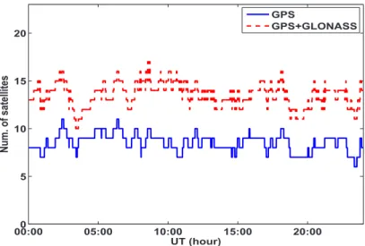
In poor observation environment (i.e., downtown area), the GPS occasionally has trouble in determining receiver positions due to the lack of the number of visible satellites (Toshiaki et al. 2000). Also, even though the number of visi- ble satellites is sufficient, the geometric arrangement of GPS

Analysis of the Combined Positioning Accuracy using GPS and GLONASS Navigation Satellites

Byung-Kyu Choi

^1†

, Kyoung-Min Roh

¹

, Sang Jeong Lee

²

1

Astronomy and Space Technology R&D Division, Korea Astronomy and Space Science Institute, Daejeon 305-348, Korea

2

Department of Electronics Engineering, Chungnam National University, Daejeon 305-764, Korea

ABSTRACT

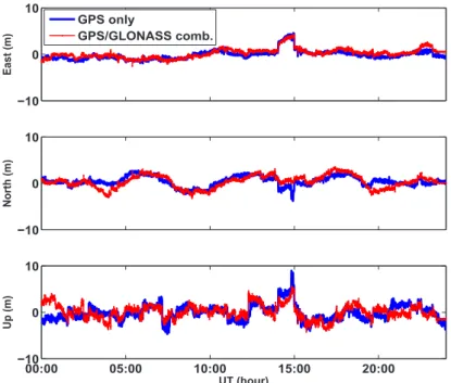
In this study, positioning results that combined the code observation information of GPS and GLONASS navigation satellites were analyzed. Especially, the distribution of GLONASS satellites observed in Korea and the combined GPS/GLONASS positioning results were presented. The GNSS data received at two reference stations (GRAS in Europe and KOHG in Goheung, Korea) during a day were processed, and the mean value and root mean square (RMS) value of the position error were calculated. The analysis results indicated that the combined GPS/GLONASS positioning did not show significantly improved performance compared to the GPS-only positioning. This could be due to the inter-system hardware bias for GPS/

GLONASS receivers, the selection of transformation parameters between reference coordinate systems, the selection of a confidence level for error analysis, or the number of visible satellites at a specific time.

Keywords: GPS, GLONASS, positioning accuracy, GNSS

satellites affects the positioning accuracy and reliability.

To complement this, studies have been conducted, which increase the number of visible satellites and positioning reliability by combining the observation data of GPS satel- lites and GLONASS satellites (Bruyninx 2007, Dodson et al.

1999, Cai & Gao 2007). The combination of GPS satellites and GLONASS satellites could improve the number of vis- ible satellites and the position dilution of precision (PDOP), compared to when only GPS satellites are used.

GLONASS satellites have large potential for precision navigation and positioning, which has been demonstrated by the International GLONASS Service Pilot Project (Zarraoa et al. 1998).

A combined positioning method, which uses the obser- vation data of GPS and GLONASS satellites, is very similar to a GPS-only positioning method. Both of the two systems are based on the principle of triangulation that considers the distance between satellite and receiver. However, the GPS and GLONASS navigation satellite systems have completely different navigation data structure, reference coordinate system, and reference time system. Therefore, to calculate the final solution by combining the observation data of the two systems, the data interpretation (e.g., satellite orbit de- termination and statistical error model) needs to be applied differently.

Kim & Park (2009) conducted a study that evaluates the Received June 03, 2013 Revised July 24, 2013 Accepted Oct 8, 2013

†

Corresponding Author E-mail: [email protected]

Tel: +82-42-865-3237 Fax: +82-42-865-5610

132 J. Korean GNSS Society 2(2), 131-137 (2013)

http://dx.doi.org/10.11003/JKGS.2013.2.2.131

orbit accuracy of satellites using the Runge-Kutta method for the orbit prediction of GLONASS satellites. Lee et al.

(2010) analyzed the orbit determination and accuracy of GLONASS satellites. Also, Park & Song (2004) derived a GLONASS measurement model, which can simultaneously use the GPS and the GLONASS, and Kang et al. (2001) used the coarse/acquisition (C/A) code and Yuma satellite orbit information to analyze the precision of absolute position- ing by combining the observation data of the GPS and the GLONASS.

In this study, an algorithm that calculates positioning results by simultaneously using the observation data of GPS and GLONASS satellites was developed, and the position accuracy was compared with that of GPS-only positioning results.

2. OUTLINE OF THE GPS AND GLONASS SYSTEMS

GPS satellites use two frequencies in the L-band (L1~1575.42MHz and L2~1227.60MHz). Each satellite has its own identification code [i.e., pseudo random noise (PRN) code], and this is an important element of the code division multiple access (CDMA) method.

On the other hand, for the GLONASS system, each satel- lite uses different frequencies. In other words, frequency division multiple access (FDMA) method is used, and it is somewhat more complicated than the GPS. GLONASS satel- lites transmit signals in two frequency bands, as shown in Eqs. (1) and (2) (Abbasian & Petovello 2010).

GLONASS satellites have large potential for precision navigation and positioning, which has been demonstrated by the International GLONASS Service Pilot Project (Zarraoa et al. 1998).

A combined positioning method, which uses the observation data of GPS and GLONASS satellites, is very similar to a GPS-only positioning method. Both of the two systems are based on the principle of triangulation that considers the distance between satellite and receiver. However, the GPS and GLONASS navigation satellite systems have completely different navigation data structure, reference coordinate system, and reference time system. Therefore, to calculate the final solution by combining the observation data of the two systems, the data interpretation (e.g., satellite orbit determination and statistical error model) needs to be applied differently.

Kim & Park

 

(2009) conducted a study that evaluates the orbit accuracy of satellites using the Runge-Kutta method for the orbit prediction of GLONASS satellites. Lee et al. (2010) analyzed the orbit determination and accuracy of GLONASS satellites. Also, Park & Song (2004) derived a GLONASS measurement model, which can simultaneously use the GPS and the GLONASS, and Kang et al. (2001) used the coarse/acquisition (C/A) code and Yuma satellite orbit information to analyze the precision of absolute positioning by combining the observation data of the GPS and the GLONASS.

In this study, an algorithm that calculates positioning results by simultaneously using the observation data of GPS and GLONASS satellites was developed, and the position accuracy was compared with that of GPS-only positioning results.

2. OUTLINE OF THE GPS AND GLONASS SYSTEMS

GPS satellites use two frequencies in the L-band (L1~1575.42MHz and L2~1227.60MHz). Each satellite has its own identification code [i.e., pseudo random noise (PRN) code], and this is an important element of the code division multiple access (CDMA) method.

On the other hand, for the GLONASS system, each satellite uses different frequencies. In other words, frequency division multiple access (FDMA) method is used, and it is somewhat more complicated than the GPS. GLONASS satellites transmit signals in two frequency bands, as shown in Eqs. (1) and (2) (Abbasian & Petovello 2010).

1

(1602 0.5625) MHz

f

L

= + × n (1)

2

(1246 0.4375) MHz

f

L

= + × n (2) where n ( n =0,1,2,...) represents the frequency channel number.

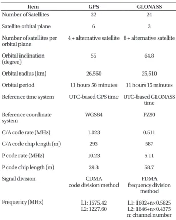
Table 1 summarizes the comparison of the GPS and GLONASS systems. As shown in the table, the two systems are basically different systems (e.g., number of satellites, reference time system, and reference coordinate system).

The broadcast ephemeris of GPS satellites is sent to users via navigation messages.

Navigation messages include orbital elements and other ephemeris information, and GPS satellites perform orbit determination using this ephemeris information. The International GNSS Service (IGS) reported that the error of GPS satellites using broadcast ephemeris is about 1 m level (http://igs.org/components/prods.html). Unlike the GPS, for the broadcast ephemeris of GLONASS satellites, velocity and acceleration components at a specific time are transmitted rather than orbital elements. Therefore, for the orbit determination of

(1)

GLONASS satellites have large potential for precision navigation and positioning, which has been demonstrated by the International GLONASS Service Pilot Project (Zarraoa et al. 1998).

A combined positioning method, which uses the observation data of GPS and GLONASS satellites, is very similar to a GPS-only positioning method. Both of the two systems are based on the principle of triangulation that considers the distance between satellite and receiver. However, the GPS and GLONASS navigation satellite systems have completely different navigation data structure, reference coordinate system, and reference time system. Therefore, to calculate the final solution by combining the observation data of the two systems, the data interpretation (e.g., satellite orbit determination and statistical error model) needs to be applied differently.

Kim & Park

 

(2009) conducted a study that evaluates the orbit accuracy of satellites using the Runge-Kutta method for the orbit prediction of GLONASS satellites. Lee et al. (2010) analyzed the orbit determination and accuracy of GLONASS satellites. Also, Park & Song (2004) derived a GLONASS measurement model, which can simultaneously use the GPS and the GLONASS, and Kang et al. (2001) used the coarse/acquisition (C/A) code and Yuma satellite orbit information to analyze the precision of absolute positioning by combining the observation data of the GPS and the GLONASS.

In this study, an algorithm that calculates positioning results by simultaneously using the observation data of GPS and GLONASS satellites was developed, and the position accuracy was compared with that of GPS-only positioning results.

2. OUTLINE OF THE GPS AND GLONASS SYSTEMS

GPS satellites use two frequencies in the L-band (L1~1575.42MHz and L2~1227.60MHz). Each satellite has its own identification code [i.e., pseudo random noise (PRN) code], and this is an important element of the code division multiple access (CDMA) method.

On the other hand, for the GLONASS system, each satellite uses different frequencies. In other words, frequency division multiple access (FDMA) method is used, and it is somewhat more complicated than the GPS. GLONASS satellites transmit signals in two frequency bands, as shown in Eqs. (1) and (2) (Abbasian & Petovello 2010).

1

(1602 0.5625) MHz

f

L

= + × n (1)

2

(1246 0.4375) MHz

f

L

= + × n (2) where n ( n =0,1,2,...) represents the frequency channel number.

Table 1 summarizes the comparison of the GPS and GLONASS systems. As shown in the table, the two systems are basically different systems (e.g., number of satellites, reference time system, and reference coordinate system).

The broadcast ephemeris of GPS satellites is sent to users via navigation messages.

Navigation messages include orbital elements and other ephemeris information, and GPS satellites perform orbit determination using this ephemeris information. The International GNSS Service (IGS) reported that the error of GPS satellites using broadcast ephemeris is about 1 m level (http://igs.org/components/prods.html). Unlike the GPS, for the broadcast ephemeris of GLONASS satellites, velocity and acceleration components at a specific time are transmitted rather than orbital elements. Therefore, for the orbit determination of

(2)

where n(n=0,1,2,...) represents the frequency channel number.

Table 1 summarizes the comparison of the GPS and GLONASS systems. As shown in the table, the two systems are basically different systems (e.g., number of satellites, reference time system, and reference coordinate system).

The broadcast ephemeris of GPS satellites is sent to users via navigation messages. Navigation messages include orbital elements and other ephemeris information, and GPS satellites perform orbit determination using this ephemeris information. The International GNSS Service (IGS) reported that the error of GPS satellites using broadcast ephemeris is about 1 m level (http://igs.org/components/prods.html).

Unlike the GPS, for the broadcast ephemeris of GLONASS satellites, velocity and acceleration components at a specific time are transmitted rather than orbital elements. Therefore,

for the orbit determination of GLONASS satellites, six orbital differential equations that were published in the GLONASS interface control document (ICD) are required, as shown in Eqs. (3-8).

GLONASS satellites, six orbital differential equations that were published in the GLONASS interface control document (ICD) are required, as shown in Eqs. (3) to (8).

dx V

x

dt = (3) dy V

y

dt = (4)

dz V

z

dt = (5)

2 2

20 32 3

3 5 2

( )

3 [1 5 ] 2

2

x e

y

dV x C a x z x V x

dt r r r

μ

μ ω ω

= − + − + + + && (6)

2 2

20 32 3

3 5 2

( )

3 [1 5 ] 2

2

y e

x

dV y C a y z y V y

dt r r r

μ

μ ω ω

= − + − + − + && (7)

2 2

3 20 5 2

( )

3 [3 5 ]

2

^e

z

a

dV z C z z z

dt r r r

μ

= − μ + − + && (8)

where, r = x

²

+ y

²

+ z

²

gravitational constant, μ = 398600.44 km s

³

/

²

, 6378136.0m a =

_e

equatorial radius of Earth, C

20

= − 1082.63 10 ×

⁻⁶

coefficient of Earth’s gravitational field of spherical harmonic expansion, ω

₃

= 7.292115 10 ×

⁻⁵

Earth’s rotation rate.

The broadcast ephemeris of GLONASS satellites is transmitted every 30 minutes (15 and 45 minutes on every hour). Thus, to determine satellite orbits at a specific time, a method for propagating orbits is needed. Therefore, in this study, the quartic Runge-Kutta equation that is recommended by the GLONASS ICD (2008) was used. The Runge-Kutta method determines satellite orbits by the numerical integration of the orbital differential equations explained earlier, as shown in Eq. (9) (Rice 1983).

1

1 ( 2 2

1 2 3 4

)

n n

6

y

+

= y + κ + κ + κ κ + (9)

where, κ

1

= hf t y ( , )

n n

2

( ,

1

)

2 2

n

h

n

hf t y κ

κ = + +

3

( ,

2

)

2 2

n

h

n

hf t y κ

κ = + +

4

( ,

3

)

n

2 h

n

hf t y κ = + + κ

In Eq. (9),

¹6

( κ

1

+ 2 κ

2

+ 2 κ κ

3

+

4

) represents the average gradient of the function, and h represents the ‘step size’. In this study, h was set to 60, considering the integration time and the satellite orbit propagation precision.

To verify the orbits of GLONASS satellites calculated using broadcast ephemeris, they were compared with the precise ephemeris provided by the IGS. Figs. 1a-d show the orbit error between the GLONASS satellite orbits calculated using broadcast ephemeris and the precise ephemeris (iglxxxxx.sp3). The results of this study were compared with the precise ephemeris, assuming that the precise ephemeris is the true value. For the GLONASS satellite

(3) (4) (5) (6) (7) (8)

where,

GLONASS satellites, six orbital differential equations that were published in the GLONASS interface control document (ICD) are required, as shown in Eqs. (3) to (8).

dx V

x

dt = (3) dy V

y

dt = (4)

dz V

z

dt = (5)

2 2

2

20 3 3

3 5 2

( )

3 [1 5 ] 2

2

x e

y

dV x C a x z x V x

dt r r r

μ

μ ω ω

= − + − + + + && (6)

2 2

2

20 3 3

3 5 2

( )

3 [1 5 ] 2

2

y e

x

dV y C a y z y V y

dt r r r

μ

μ ω ω

= − + − + − + && (7)

2 2

3 20 5 2

( )

3 [3 5 ]

2

^e

z

a

dV z C z z z

dt r r r

μ

= − μ + − + && (8)

where, r = x y z

²

+ +

^{2 2}

gravitational constant, μ = 398600.44 km s

³

/

²

, 6378136.0m a =

e

equatorial radius of Earth, C

20

= − 1082.63 10 ×

⁻⁶

coefficient of Earth’s gravitational field of spherical harmonic expansion, ω

3

= 7.292115 10 ×

⁻⁵

Earth’s rotation rate.

The broadcast ephemeris of GLONASS satellites is transmitted every 30 minutes (15 and 45 minutes on every hour). Thus, to determine satellite orbits at a specific time, a method for propagating orbits is needed. Therefore, in this study, the quartic Runge-Kutta equation that is recommended by the GLONASS ICD (2008) was used. The Runge-Kutta method determines satellite orbits by the numerical integration of the orbital differential equations explained earlier, as shown in Eq. (9) (Rice 1983).

1

1 ( 2 2

1 2 3 4

)

n n

6

y

₊

= + y κ + κ + κ κ + (9)

where, κ =

₁

hf t y ( , )

n n

2

( ,

1

)

2 2

n

h

n

hf t y κ

κ = + +

3

( ,

2

)

2 2

n

h

n

hf t y κ

κ = + +

4

( ,

3

)

n

2 h

n

hf t y

κ = + + κ

In Eq. (9),

¹6

( κ

1

+ 2 κ

2

+ 2 κ κ

3

+

4

) represents the average gradient of the function, and h represents the ‘step size’. In this study, h was set to 60, considering the integration time and the satellite orbit propagation precision.

To verify the orbits of GLONASS satellites calculated using broadcast ephemeris, they were compared with the precise ephemeris provided by the IGS. Figs. 1a-d show the orbit error between the GLONASS satellite orbits calculated using broadcast ephemeris and the precise ephemeris (iglxxxxx.sp3). The results of this study were compared with the precise ephemeris, assuming that the precise ephemeris is the true value. For the GLONASS satellite

gravitational constant,

GLONASS satellites, six orbital differential equations that were published in the GLONASS interface control document (ICD) are required, as shown in Eqs. (3) to (8).

dx V

x

dt = (3) dy V

y

dt = (4)

dz V

z

dt = (5)

2 2

2

20 3 3

3 5 2

( )

3 [1 5 ] 2

2

x e

y

dV x C a x z x V x

dt r r r

μ

μ ω ω

= − + − + + + && (6)

2 2

2

20 3 3

3 5 2

( )

3 [1 5 ] 2

2

y e

x

dV y C a y z y V y

dt r r r

μ μ ω ω

= − + − + − + && (7)

2 2

3 20 5 2

( )

3 [3 5 ]

2

^e

z

a

dV z C z z z

dt r r r

μ

= − μ + − + && (8)

where, r = x

²

+ y

²

+ z

²

gravitational constant, μ = 398600.44 km s

³

/

²

, 6378136.0m a =

e

equatorial radius of Earth, C

20

= − 1082.63 10 ×

⁻⁶

coefficient of Earth’s gravitational field of spherical harmonic expansion, ω

3

= 7.292115 10 ×

⁻⁵

Earth’s rotation rate.

The broadcast ephemeris of GLONASS satellites is transmitted every 30 minutes (15 and 45 minutes on every hour). Thus, to determine satellite orbits at a specific time, a method for propagating orbits is needed. Therefore, in this study, the quartic Runge-Kutta equation that is recommended by the GLONASS ICD (2008) was used. The Runge-Kutta method determines satellite orbits by the numerical integration of the orbital differential equations explained earlier, as shown in Eq. (9) (Rice 1983).

1

1 ( 2 2

1 2 3 4

)

n n

6

y

+

= y + κ + κ + κ κ + (9)

where, κ =

₁

hf t y ( , )

n n

2

( ,

1

)

2 2

n

h

n

hf t y κ

κ = + +

3

( ,

2

)

2 2

n

h

n

hf t y κ

κ = + +

4

( ,

3

)

n

2 h

n

hf t y

κ = + + κ

In Eq. (9),

¹6

( κ

1

+ 2 κ

2

+ 2 κ κ

3

+

4

) represents the average gradient of the function, and h represents the ‘step size’. In this study, h was set to 60, considering the integration time and the satellite orbit propagation precision.

To verify the orbits of GLONASS satellites calculated using broadcast ephemeris, they were compared with the precise ephemeris provided by the IGS. Figs. 1a-d show the orbit error between the GLONASS satellite orbits calculated using broadcast ephemeris and the precise ephemeris (iglxxxxx.sp3). The results of this study were compared with the precise ephemeris, assuming that the precise ephemeris is the true value. For the GLONASS satellite

= 398600.44km

³

/ s

²

, a

_e

= 6378136.0m equatorial radius of Earth, C

₂₀

= -1082.63 x 10

^-6

coefficient of Earth’s gravitational field of spherical harmonic expansion,

GLONASS satellites, six orbital differential equations that were published in the GLONASS interface control document (ICD) are required, as shown in Eqs. (3) to (8).

dx V

x

dt = (3) dy V

y

dt = (4)

dz V

z

dt = (5)

2 2

20 32 3

3 5 2

( )

3 [1 5 ] 2

2

x e

y

dV x C a x z x V x

dt r r r

μ

μ ω ω

= − + − + + + && (6)

2 2

20 32 3

3

3 ( )

5

[1 5

2

] 2

2

y e

x

dV y C a y z y V y

dt r r r

μ

μ ω ω

= − + − + − + && (7)

2 2

3 20 5 2

( )

3 [3 5 ]

2

^e

z

a

dV z C z z z

dt r r r

μ

= − μ + − + && (8)

where, r = x

²

+ y

²

+ z

²

gravitational constant, μ = 398600.44 km s

³

/

²

, 6378136.0m a =

_e

equatorial radius of Earth, C

20

= − 1082.63 10 ×

⁻⁶

coefficient of Earth’s gravitational field of spherical harmonic expansion, ω

3

= 7.292115 10 ×

⁻⁵

Earth’s rotation rate.

The broadcast ephemeris of GLONASS satellites is transmitted every 30 minutes (15 and 45 minutes on every hour). Thus, to determine satellite orbits at a specific time, a method for propagating orbits is needed. Therefore, in this study, the quartic Runge-Kutta equation that is recommended by the GLONASS ICD (2008) was used. The Runge-Kutta method determines satellite orbits by the numerical integration of the orbital differential equations explained earlier, as shown in Eq. (9) (Rice 1983).

1

1 ( 2 2

1 2 3 4

)

n n

6

y

₊

= y + κ + κ + κ κ + (9)

where, κ =

1

hf t y ( , )

n n

2

( ,

1

)

2 2

n

h

n

hf t y κ

κ = + +

3

( ,

2

)

2 2

n

h

n

hf t y κ

κ = + +

4

( ,

3

)

n

2 h

n

hf t y

κ = + + κ

In Eq. (9),

¹6

( κ

1

+ 2 κ

2

+ 2 κ κ

3

+

4

) represents the average gradient of the function, and h represents the ‘step size’. In this study, h was set to 60, considering the integration time and the satellite orbit propagation precision.

To verify the orbits of GLONASS satellites calculated using broadcast ephemeris, they were compared with the precise ephemeris provided by the IGS. Figs. 1a-d show the orbit error between the GLONASS satellite orbits calculated using broadcast ephemeris and the precise ephemeris (iglxxxxx.sp3). The results of this study were compared with the precise ephemeris, assuming that the precise ephemeris is the true value. For the GLONASS satellite

Earth’s rotation rate.

The broadcast ephemeris of GLONASS satellites is transmitted every 30 minutes (15 and 45 minutes on every Table 1. Comparison of the GPS and GLONASS systems (Reference week number: 1698).

Item GPS GLONASS

Number of Satellites Satellite orbital plane Number of satellites per orbital plane Orbital inclination (degree) Orbital radius (km) Orbital period Reference time system

Reference coordinate system

C/A code rate (MHz) C/A code chip length (m) P code rate (MHz) P code chip length (m) Signal division

Frequency (MHz)

32 6 4 + alternative satellite

55

26,560 11 hours 58 minutes UTC-based GPS time

WGS84

1.023 293 10.23

29.3 CDMA code division method

L1: 1575.42 L2: 1227.60

24 3 8 + alternative satellite

64.8

25,510 11 hours 15 minutes UTC-based GLONASS

time PZ90

0.511 587 5.11 58.7 frequency division FDMA

method

L1: 1602+n×0.5625

L2: 1646+n×0.4375

n: channel number

Byung-Kyu Choi et al. Combined Positioning using GPS and GLONASS 133

http://www.gnss.or.kr hour). Thus, to determine satellite orbits at a specific time, a method for propagating orbits is needed. Therefore, in this study, the quartic Runge-Kutta equation that is recommended by the GLONASS ICD (2008) was used. The Runge-Kutta method determines satellite orbits by the numerical integration of the orbital differential equations explained earlier, as shown in Eq. (9) (Rice 1983).

GLONASS satellites, six orbital differential equations that were published in the GLONASS interface control document (ICD) are required, as shown in Eqs. (3) to (8).

dx V

x

dt = (3) dy V

y

dt = (4)

dz V

z

dt = (5)

2 2

2

20 3 3

3 5 2

( )

3 [1 5 ] 2

2

x e

y

dV x C a x z x V x

dt r r r

μ

μ ω ω

= − + − + + + && (6)

2 2

20 32 3

3 5 2

( )

3 [1 5 ] 2

2

y e

x

dV y C a y z y V y

dt r r r

μ μ ω ω

= − + − + − + && (7)

2 2

3 20 5 2

( )

3 [3 5 ]

2

^e

z

a

dV z C z z z

dt r r r

μ

= − μ + − + && (8)

where, r = x

²

+ y

²

+ z

²

gravitational constant, μ = 398600.44 km s

³

/

²

, 6378136.0m a =

_e

equatorial radius of Earth, C

₂₀

= − 1082.63 10 ×

⁻⁶

coefficient of Earth’s gravitational field of spherical harmonic expansion, ω

₃

= 7.292115 10 ×

⁻⁵

Earth’s rotation rate.

The broadcast ephemeris of GLONASS satellites is transmitted every 30 minutes (15 and 45 minutes on every hour). Thus, to determine satellite orbits at a specific time, a method for propagating orbits is needed. Therefore, in this study, the quartic Runge-Kutta equation that is recommended by the GLONASS ICD (2008) was used. The Runge-Kutta method determines satellite orbits by the numerical integration of the orbital differential equations explained earlier, as shown in Eq. (9) (Rice 1983).

1

1 ( 2 2

1 2 3 4

)

n n

6

y

+

= y + κ + κ + κ κ + (9)

where, κ

₁

= hf t y ( , )

_{n n}

2

( ,

1

)

2 2

n

h

n

hf t y κ

κ = + +

3

( ,

2

)

2 2

n

h

n

hf t y κ

κ = + +

4

( ,

3

)

n

2 h

n

hf t y κ = + + κ

In Eq. (9),

¹₆

( κ

₁

+ 2 κ

₂

+ 2 κ κ

₃

+

₄

) represents the average gradient of the function, and h represents the ‘step size’. In this study, h was set to 60, considering the integration time and the satellite orbit propagation precision.

To verify the orbits of GLONASS satellites calculated using broadcast ephemeris, they were compared with the precise ephemeris provided by the IGS. Figs. 1a-d show the orbit error between the GLONASS satellite orbits calculated using broadcast ephemeris and the precise ephemeris (iglxxxxx.sp3). The results of this study were compared with the precise ephemeris, assuming that the precise ephemeris is the true value. For the GLONASS satellite

(9) where,

GLONASS satellites, six orbital differential equations that were published in the GLONASS interface control document (ICD) are required, as shown in Eqs. (3) to (8).

dx V

x

dt = (3) dy V

y

dt = (4)

dz V

z

dt = (5)

2 2

20 32 3

3 5 2

( )

3 [1 5 ] 2

2

x e

y

dV x C a x z x V x

dt r r r

μ μ ω ω

= − + − + + + && (6)

2 2

20 32 3

3 5 2

( )

3 [1 5 ] 2

2

y e

x

dV y C a y z y V y

dt r r r

μ

μ ω ω

= − + − + − + && (7)

2 2

3 20 5 2

3 ( ) [3 5 ]

2

^e

z

a

dV z C z z z

dt r r r

μ

= − μ + − + && (8)

where, r = x

²

+ y

²

+ z

²

gravitational constant, μ = 398600.44 km s

³

/

²

, 6378136.0m a =

_e

equatorial radius of Earth, C

20

= − 1082.63 10 ×

⁻⁶

coefficient of Earth’s gravitational field of spherical harmonic expansion, ω

₃

= 7.292115 10 ×

⁻⁵

Earth’s rotation rate.

The broadcast ephemeris of GLONASS satellites is transmitted every 30 minutes (15 and 45 minutes on every hour). Thus, to determine satellite orbits at a specific time, a method for propagating orbits is needed. Therefore, in this study, the quartic Runge-Kutta equation that is recommended by the GLONASS ICD (2008) was used. The Runge-Kutta method determines satellite orbits by the numerical integration of the orbital differential equations explained earlier, as shown in Eq. (9) (Rice 1983).

1

1 ( 2 2

1 2 3 4

)

n n

6

y

+

= y + κ + κ + κ κ + (9)

where, κ

1

= hf t y ( , )

n n

2

( ,

1

)

2 2

n

h

n

hf t y κ

κ = + +

3

( ,

2

)

2 2

n

h

n

hf t y κ

κ = + +

4

( ,

3

)

n

2 h

n

hf t y

κ = + + κ

In Eq. (9),

¹6

( κ

1

+ 2 κ

2

+ 2 κ κ

3

+

4

) represents the average gradient of the function, and h represents the ‘step size’. In this study, h was set to 60, considering the integration time and the satellite orbit propagation precision.

To verify the orbits of GLONASS satellites calculated using broadcast ephemeris, they were compared with the precise ephemeris provided by the IGS. Figs. 1a-d show the orbit error between the GLONASS satellite orbits calculated using broadcast ephemeris and the precise ephemeris (iglxxxxx.sp3). The results of this study were compared with the precise ephemeris, assuming that the precise ephemeris is the true value. For the GLONASS satellite

In Eq. (9),

GLONASS satellites, six orbital differential equations that were published in the GLONASS interface control document (ICD) are required, as shown in Eqs. (3) to (8).

dx V

x

dt = (3) dy V

y

dt = (4)

dz V

z

dt = (5)

2 2

20 32 3

3 5 2

( )

3 [1 5 ] 2

2

x e

y

dV x C a x z x V x

dt r r r

μ

μ ω ω

= − + − + + + && (6)

2 2

20 32 3

3 5 2

3 ( ) [1 5 ] 2

2

y e

x

dV y C a y z y V y

dt r r r

μ

μ ω ω

= − + − + − + && (7)

2 2

3 20 5 2

( )

3 [3 5 ]

2

^e

z

a

dV z C z z z

dt r r r

μ

= − μ + − + && (8)

where, r = x

²

+ y

²

+ z

²

gravitational constant, μ = 398600.44 km s

³

/

²

, 6378136.0m a =

_e

equatorial radius of Earth, C

₂₀

= − 1082.63 10 ×

⁻⁶

coefficient of Earth’s gravitational field of spherical harmonic expansion, ω

₃

= 7.292115 10 ×

⁻⁵

Earth’s rotation rate.

The broadcast ephemeris of GLONASS satellites is transmitted every 30 minutes (15 and 45 minutes on every hour). Thus, to determine satellite orbits at a specific time, a method for propagating orbits is needed. Therefore, in this study, the quartic Runge-Kutta equation that is recommended by the GLONASS ICD (2008) was used. The Runge-Kutta method determines satellite orbits by the numerical integration of the orbital differential equations explained earlier, as shown in Eq. (9) (Rice 1983).

1

1 ( 2 2

1 2 3 4

)

n n

6

y

₊

= y + κ + κ + κ κ + (9)

where, κ

₁

= hf t y ( , )

_{n n}

2

( ,

1

)

2 2

n

h

n

hf t y κ

κ = + +

3

( ,

2

)

2 2

n

h

n

hf t y κ

κ = + +

4

( ,

3

)

n

2 h

n

hf t y

κ = + + κ

In Eq. (9),

¹6

( κ

1

+ 2 κ

2

+ 2 κ κ

3

+

4

) represents the average gradient of the function, and h represents the ‘step size’. In this study, h was set to 60, considering the integration time and the satellite orbit propagation precision.

To verify the orbits of GLONASS satellites calculated using broadcast ephemeris, they were compared with the precise ephemeris provided by the IGS. Figs. 1a-d show the orbit error between the GLONASS satellite orbits calculated using broadcast ephemeris and the precise ephemeris (iglxxxxx.sp3). The results of this study were compared with the precise ephemeris, assuming that the precise ephemeris is the true value. For the GLONASS satellite

represents the average gradient of the function, and h represents the ‘step size’. In this study, h was set to 60, considering the integration time and the satellite orbit propagation precision.

To verify the orbits of GLONASS satellites calculated using broadcast ephemeris, they were compared with the precise ephemeris provided by the IGS. Figs. 1a-d show the orbit error between the GLONASS satellite orbits calculated using broadcast ephemeris and the precise ephemeris (iglxxxxx.sp3). The results of this study were compared with the precise ephemeris, assuming that the precise ephemeris is the true value. For the GLONASS satellite orbits calculated using broadcast ephemeris, the average RMS value for each component was generally 2~3 m level, although there was slight difference among satellites.

3. COMBINED GPS/GLONASS POSITIONING METHOD AND RESULT VERIFICATION

To determine user positions using only the L1 code observation values of the GPS satellites and the GLONASS satellites, the weighted least squares method was applied (Tarrio et al. 2011).

orbits calculated using broadcast ephemeris, the average RMS value for each component was generally 2~3 m level, although there was slight difference among satellites.

3. COMBINED GPS/GLONASS POSITIONING METHOD AND RESULT VERIFICATION

To determine user positions using only the L1 code observation values of the GPS satellites and the GLONASS satellites, the weighted least squares method was applied (Tarrio et al. 2011).

(

^T

)

1 ^T

x = H WH H Wv

⁻

(10) where H is the design matrix, W is the weight matrix for the GPS satellites and the GLONASS satellites, and v is the pseudorange residual vector. The state vector of the final solution is x = Δ Δ Δ Δ [ , , , x y z t

_gps

, Δ t

_glo

] , and it consists of the position error in the World Geodetic System (WGS84) reference coordinate, the receiver clock error related with the GPS time, and the receiver clock error related with the GLONASS time.

1 1 1

2 2 2

1 1 1

1 0 1 0 1 0 0 1 0 1

gps gps gps

x y z

gps gps gps

x y z

gpsN gpsN gpsN

x y z

glo glo glo

x y z

gloM gloM gloM

x y z

H

α α α

α α α

α α α

α α α

α α α

⎡ ⎤

⎢ ⎥

⎢ ⎥

⎢ ⎥

⎢ ⎥

= ⎢ ⎥

⎢ ⎥

⎢ ⎥

⎢ ⎥

⎢ ⎥

⎣ ⎦

M M M M M

M M M M M

(11)

The data processing time was based on the Universal Time Coordinated (UTC), and the design matrix H was constructed as shown in Eq. (11).

For the reference coordinate system, the GLONASS system uses PZ90, and the GPS system uses WGS84. Therefore, to obtain consistent positioning results, transformation between the different coordinate systems is needed. For the transformation between the reference coordinate systems (i.e., Helmert transformation), total seven parameters are required such as three translation parameters ( T T T ), three rotation parameters

_X

, ,

_{Y Z}

( R R R ), and a scale factor (S). The transformation equation is shown in Eq. (12)

_X

, ,

_{Y Z}

(Boucher & Altamimi 2001).

84 90 90

X Z Y

Y Z X

Z Y X

WGS PZ PZ

X X T S R R X

Y Y T R S R Y

Z Z T R R S Z

⎡ ⎤ ⎡ ⎤ ⎡ ⎤ ⎡ − ⎤ ⎡ ⎤

⎢ ⎥ = ⎢ ⎥ + ⎢ ⎥ ⎢ + − ⎥ ⎢ ⎥

⎢ ⎥ ⎢ ⎥ ⎢ ⎥ ⎢ ⎥ ⎢ ⎥

⎢ ⎥ ⎢ ⎥ ⎢ ⎥ ⎢ − ⎥ ⎢ ⎥

⎣ ⎦ ⎣ ⎦ ⎣ ⎦ ⎣ ⎦ ⎣ ⎦

(12)

To compare and verify the GPS-only positioning results and the combined GPS/GLONASS positioning results, the data from two GNSS reference stations (GRAS in Europe and KOHG in Goheung, Korea) were processed. For data processing, the data received at the reference stations during a day on July 22, 2012 was used.

(10)

where H is the design matrix, W is the weight matrix for the GPS satellites and the GLONASS satellites, and is the pseudorange residual vector. The state vector of the final solution is

orbits calculated using broadcast ephemeris, the average RMS value for each component was generally 2~3 m level, although there was slight difference among satellites.

3. COMBINED GPS/GLONASS POSITIONING METHOD AND RESULT VERIFICATION

To determine user positions using only the L1 code observation values of the GPS satellites and the GLONASS satellites, the weighted least squares method was applied (Tarrio et al. 2011).

(

^T

)

1 ^T

x = H WH H Wv

⁻

(10) where H is the design matrix, W is the weight matrix for the GPS satellites and the GLONASS satellites, and v is the pseudorange residual vector. The state vector of the final solution is x = Δ Δ Δ Δ [ , , , x y z t

_gps

, Δ t

_glo

] , and it consists of the position error in the World Geodetic System (WGS84) reference coordinate, the receiver clock error related with the GPS time, and the receiver clock error related with the GLONASS time.

1 1 1

2 2 2

1 1 1

1 0 1 0

1 0 0 1 0 1

gps gps gps

x y z

gps gps gps

x y z

gpsN gpsN gpsN

x y z

glo glo glo

x y z

gloM gloM gloM

x y z

H

α α α

α α α

α α α

α α α

α α α

⎡ ⎤

⎢ ⎥

⎢ ⎥

⎢ ⎥

⎢ ⎥

= ⎢ ⎥

⎢ ⎥

⎢ ⎥

⎢ ⎥

⎢ ⎥

⎣ ⎦

M M M M M

M M M M M

(11)

The data processing time was based on the Universal Time Coordinated (UTC), and the design matrix H was constructed as shown in Eq. (11).

For the reference coordinate system, the GLONASS system uses PZ90, and the GPS system uses WGS84. Therefore, to obtain consistent positioning results, transformation between the different coordinate systems is needed. For the transformation between the reference coordinate systems (i.e., Helmert transformation), total seven parameters are required such as three translation parameters ( T T T ), three rotation parameters

_X

, ,

_{Y Z}

( R R R ), and a scale factor (S). The transformation equation is shown in Eq. (12)

_X

, ,

_{Y Z}

(Boucher & Altamimi 2001).

84 90 90

X Z Y

Y Z X

Z Y X

WGS PZ PZ

X X T S R R X

Y Y T R S R Y

Z Z T R R S Z

⎡ ⎤ ⎡ ⎤ ⎡ ⎤ ⎡ − ⎤ ⎡ ⎤

⎢ ⎥ = ⎢ ⎥ + ⎢ ⎥ ⎢ + − ⎥ ⎢ ⎥

⎢ ⎥ ⎢ ⎥ ⎢ ⎥ ⎢ ⎥ ⎢ ⎥

⎢ ⎥ ⎢ ⎥ ⎢ ⎥ ⎢ − ⎥ ⎢ ⎥

⎣ ⎦ ⎣ ⎦ ⎣ ⎦ ⎣ ⎦ ⎣ ⎦

(12)

To compare and verify the GPS-only positioning results and the combined GPS/GLONASS positioning results, the data from two GNSS reference stations (GRAS in Europe and KOHG in Goheung, Korea) were processed. For data processing, the data received at the reference stations during a day on July 22, 2012 was used.

, and it consists of the position error in the World Geodetic System (WGS84) Fig. 1. Orbit error between the GLONASS satellite orbits calculated using

broadcast ephemeris and the precise ephemeris: (a) GLONASS satellite 1, (b)

GLONASS satellite 5, (c) GLONASS satellite 21, and (d) GLONASS satellite 24.