Proofs of Utkin's Theorem for MIMO Uncertain Integral Linear Systems
Jung-Hoon Lee*★
Abstract
The uncertain integral linear system is the integral-augmented uncertain system to improve the resultant performance. In this note, for a MI(Multi Input) uncertain integral linear case, Utkin's theorem is proved clearly and comparatively. With respect to the two transformations(diagonalizations), the equation of the sliding mode is invariant. By using the results of this note, in the SMC for MIMO uncertain integral linear systems, the existence condition of the sliding mode on the predetermined sliding surface is easily proved.
The effectiveness of the main results is verified through an illustrative example and simulation study.
Key words: Utkin’s theorem, Sliding mode control, Variable structure system, Diagonalization method, Transformation method
*ERI, Dept. of Control & Instrum. Eng., Gyeongsang National University,
★Corresponding author, email:[email protected], phone:+82-55-772-1742
Manuscript received 2014; reviced: 2014; accepted 2014
I. Introduction
Recently the integral action is augmented to the variable structure system or sliding mode control to improve the output performance[1]-[12]. Concerning introduction of an integral action to the VSS so-called the integral variable structure system(IVSS), the performance of the zero steady state error and/or no reaching phase can be obtained[1]-[12], while it may exists in the digital implementation of the conventional VSS. For canonical SISO systems, the output error is integrated only to improve the steady state performance against external disturbances in [1] and [2]. In the cases of Choi and Chang, the sliding surfaces are integrated itself for control of multi-input systems[4][7]. In [8], the integral action
as function of the low pass filter is employed to reduce the chattering in the control input. In [9], the time varying sliding surfaces are presented to remove the reaching phase. In [3] and [5], the integral state with a special initial condition is augmented to the conventional VSS in order to completely remove the reaching phase. The integral-augmented uncertain linear system is called as the uncertain integral linear system to improve the resultant performance.
To take the advantages of the sliding mode on the predetermined sliding surface in the VSS or SMC, the existence condition of the sliding mode,
⋅ for the MI(multi input) linear case is satisfied. Therefore the existence condition of the sliding mode must be proved. For the linear MI case, a few control design method was studied, those are hierarchical control methodology[13][15], diagonalization methods[13][14][22][23], simplex algorithm[28], Lyapunov approach[23][29] and etc.
Only the results of the derivative of the Lyapunov function is negative, i,e. is obtained when
. The two methodologies to prove the existence condition of the sliding mode on the sliding surface were presented for MI uncertain
nonlinear systems by Utkin[13]. Those two methodologies are the control input transformation and sliding surface transformation. The proof of Utkin’s theroem is necessary for proving existence condition of the sliding mode. the But the proof is not sufficient. DeCarlo, Zak, and Matthews reviewed and tried to prove Utkin's invariance theorem. But, the proof is also not clear. The control input transformation without uncertainties and disturbance is used by Zak and Hui In [22]. But, they did not prove for the explicit control input transformation under uncertainties and disturbance. The sliding surface transformation was mentioned by Su, Drakunov, and Ozguner in [29]. In the case of the MI uncertain integral linear system, the proof of Utkin’s theorem is necessary to prove the existence condition of the sliding mode on the predetermined sliding surface.
In this paper, a proof of Utkin's theorem is presented for MI uncertain integral linear systems.
The invariance theorem with respect to the two transformation methods so called the two diagonalization methods are proved clearly and comparatively for MI uncertain integral linear systems. By using the results of this note, in the SMC for a MIMO uncertain integral linear system, the existence condition of the sliding mode on the predetermined sliding surface is easily proved. A design example and simulation study shows usefulness of the main results.
II. Main Results of Proofs of Utkin's Theorem for MI Uncertain Integral
Linear Systems
The invariant theorem of Utkin's for MI systems is as follows[13][14]:
Theorem 1: The equation of the sliding mode is invariant with respect to the two nonlinear transformations, i.e. the control input transformation and sliding surface transformation:
⋅
⋅
(1)
for det≠ and det≠ .
The theorem means that the sliding mode equation
is governed by the original (1) if the components of the controlled vector undergo discontinuity on the new surface or the components of the new control vector undergo discontinuity on the already chosen surface , that is
⇔ . Thus the performances designed in (1) can be guaranteed by the sliding mode on the new surface . For a MI uncertain linear system:
∆ ∆ ∆ (2) where ∈ is the state, ∈ is the control input, ∈ × is the nominal system matrix,
∈ × is the nominal input matrix, ∆ and
∆ are the system matrix uncertainty and input matrix uncertainty, those are bounded, and ∆
is bounded external disturbance, respectively.
For use later, an integral state for the integral linear systems is augmented as follows:
∞
(3)
where for non zero
and
(4) Then, the integral sliding surface becomes
(5)
For the coefficient matrix of the sliding surface , the following assumptions are made.
Assumption 1:
has the full rank and its inverse Assumption 2:
∆ ∆ . ∆ is diagonal and
∆ ≤
Assumption 3:
∆′ ∆ . ∆′ is diagonal and
∆′ ≤
The VSS control input is as follows:
⋅ ∆⋅ ∆⋅ (6) where is a constant gain, ∆ ∆
is a
state dependent switching gain, ∆ ∆
is a
switching gain.
(7)
∆
≥ m in ∆ m ax∆ ∆
≤ m in ∆
m in ∆ ∆
(8)
∆
≥ m in ∆ m ax∆
≤ m in ∆ m in∆
(9)
where min⋅ means the minimum value function and max⋅ implies the maximum value function.
2.1 control input transformation[15][17][23]
The control input is transformed as
⋅
⋅ ∆ ∆
⋅ ∆ ∆
(10) Then, the real dynamics of , i.e. the time derivative of is as follows:
∆ ∆ ∆
∆ ∆ ∆
∆ ∆
∆ ∆′
∆∆ ∆ ∆∆
(11) By (7), the real dynamics of becomes
∆ ∆ ∆′∆
∆ ∆ ∆
(12)
By (8) and (9), then one can obtain the following equation
⋅ (13) The existence condition of the sliding mode is proved. The equation of the sliding mode, i.e. the sliding surface is invariant to the control input transformation
2.2 sliding surface transformation[15][17][24]
⋅ (14) The transformation matrix is selected as
. In [14], its proof is not sufficient.
Now, the VSS control input is taken as follows:
⋅ ∆⋅ ∆⋅ (15) where
(16)
∆
≥ m in ∆′
m ax ∆ ∆ ′
≤ m in ∆′
m in ∆ ∆′
(17)
∆
≥ min ∆′ max ∆
≤ min ∆′ min ∆
(18)
The real dynamics of the sliding surface, i.e. the time derivative of becomes
∆ ∆
∆
∆ ∆′
∆
∆ ∆′ ∆
∆ ∆
∆
∆′ ∆′∆
∆ ∆′
(19) By (16), then the real dynamics of becomes
∆ ∆′ ∆′∆
∆ ∆′∆
(20) In [23], without uncertainty and disturbance, it is mentioned that the sliding surface transformation would diagonalize the control coefficient matrix to the dynamics for and only the is proved when .
From (20) and by (17) and (18), the following equation is obtained as
⋅ (21)
If the sliding mode equation , then
since ≠ . The inverse augment also holds, therefore the both sliding surfaces are equal i.e.,
, which completes the proof of Theorem 1.
The sliding mode equation i.e. the sliding surface
is the same as that of . To compare the control inputs, and , the form is the same but the gains of are multiplied by . The both methods equivalently diagonalize the system, so those are called the diagonalization methods. By using the results of this note, in the SMC for MIMO uncertain integral linear systems, the existence condition of the sliding mode on the predetermined sliding surface is easily proved.
Ⅲ. Design Example and Simulation Studies
3.1 Plant
Consider a fifth-order system described by the state equation which is slightly modified from that in [30]
± ±
±
± ±
±
±
±
±
±
(22) where the nominal parameter and , matched uncertainties ∆ and ∆ , and disturbance ∆
are
,
, ∆
± ±
±
± ±
±
,
∆
±
±
∆
±
±
(23)
3.2 An Example of Integral Case The integral state is augmented as follows:
(24)
The coefficient of the sliding surface is determined as
and
(25) 1) control input transformation
∆ ∆
(26)
Then, the real dynamics of , i.e. the time derivative of is as follows:
∆ ∆
∆∆∆ ∆∆
(27) where
∆ ∆
±
±
(28)
Thus, Assumption A1 is satisfied. By letting the constant gain
(29) then the real dynamics of becomes
∆ ∆ ∆∆
∆ ∆∆ (30) If one takes the switching gain as design parameters
if i f ,
i f i f , i f i f
i f i f ,
i f if , ∆ i f if
i f if , i f i f ,
i f if i f i f ,
i f if , ∆ i f if
Fig. 1 Five state output responses, , , , , and
Fig. 2 Two real trajectories and ideal trajectories on
- plane(upper) and - plane(below)
(31) then one can obtain the following equation
⋅ (32)
The existence condition of the sliding mode is proved. The equation of the sliding mode, i.e. the sliding surface is invariant to the control input transformation. The simulation is carried out under
0.1[msec] sampling time and with
initial state, by means of Fortran language. Fig. 1 shows the five state output responses, , , , , and . Fig. 2 shows the
two real trajectories and ideal trajectories on on -
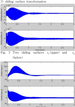
plane(upper) and - plane(below). The controlled system slides from the beginning as shown in these figures. The two sliding surfaces and two control inputs are depicted in Fig. 3 and Fig. 4, respectively.
2) sliding surface transformation
Fig. 3 Two sliding surfaces (upper) and (below)
Fig.4 Two control inputs (upper) and (below)
⋅
(33) Now, the VSS control input are taken as follows:
⋅ ∆⋅ ∆⋅ (34) The real dynamics of the sliding surface, i.e. the time derivative of becomes
∆
∆′ ∆′∆ ∆
∆′∆
(35) By letting gain
(36) then the real dynamics of becomes
∆ ∆′ ∆′∆
∆ ∆′∆
(37)
Fig. 5 Five state output responses, , , , , and
Fig. 6 Two trajectories and two ideal trajectories on
- plane(upper) and - plane(below)
∆′ ∆
±
±
(38)
Thus, Assumption A2 is satisfied. If one takes the switching gains as follows
i f if , i f i f
i f if
i f if
i f if , ∆ i f if
i f i f i f i f ,
i f i f
i f i f i f i f ,
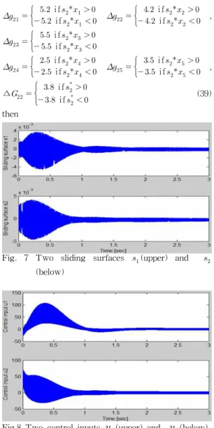
∆ if i f (39) then
Fig. 7 Two sliding surfaces (upper) and (below)
Fig.8 Two control inputs (upper) and (below)
⋅ (40)
If , then . The inverse augment also holds. The switching gains in (63) can be obtained
also from (28) by multiplying
. The simulation is carried out under 1[msec]
sampling time and with initial condition. Fig. 5 shows the five state output responses, , , , , and . Those are almost identical to Fig. 1 because the sliding surface
is equal and the continuous gains and discontinuous gains of the both controls, and
are equal. Fig. 6 shows the two real trajectories and ideal trajectories on on - plane(upper) and
- plane(below). The controlled system slides from the beginning as shown in these figures. The two sliding surfaces and two control inputs are depicted in Fig. 7 and Fig. 8, respectively.
Ⅳ. Conclusions
In this note, the invariant theorem of Utkin is rigorously proved for MI uncertain integral linear systems. The invariance theorem of the two diagonal methods i.e., the control input transformation and sliding surface transformation is proved clearly and comparatively. Therefore, the equation of the sliding mode, i.e., the sliding surface is invariant with respect to the two diagonalization methods. These two methods diagonalize the input system of the real sliding dynamics of the sliding surface or so that the existence condition of the sliding mode on the predetermined sliding surface is easily proved. During the proof of Utkin's theorem for MI uncertain integral linear systems, the design rules of both control inputs are proposed.
Through an illustrative example and simulation study, the effectiveness of the proposed main results is verified. The same results of the outputs by the two diagonalization methods are obtained. The equation of the sliding mode, i.e., the sliding surface is invariant with respect to the two diagonalization methods for MI uncertain integral linear systems.
By using the results of this note, in the SMC for a MIMO uncertain integral linear system, the existence condition of the sliding mode on the predetermined sliding surface is easily proved
References
[1] T. L. Chern and Y. C. Wu, "Design of Integral Variable Structure Controller and Application to Electrohydraulic Velocity Servosystems, lEE Proceedings-D, vol. 138, no.5, pp.439-444, 1991.
[2] T. L. Chern and Y. C. Wu, "An Optimal
Variable Structure Control with Integral Compensation for Electrohydraulic Position Servo Control Systems, IEEE Trans.
Industrial Electronics, vol. 39, no. 5, pp.460-463, 1992.
[3]J. H. Lee and M. J. Youn, "An Integral-Augmented Optimal Variable Structure control for Uncertain dynamical SISO System, KIEE(The Korean Institute of Electrical Engineers), vol.43, no.8, pp.1333-1351, 1994.
[4]H. H. Choi, " LMI-Based Sliding Surface Design for Integral Sliding Mode Control of Mismatched Uncertain Systems, IEEE T.
Automatic Control, vol.52, no.2 pp736-742, 2007.
[5]J. H. Lee, Design of Integral-Augmented Optimal Variable Structure Controllers. Ph. D.
Dissertation, KAIST, 1995.
[6] H. C. Tseng and P. V. Kokotovic, "Tracking and Disturbance Rejection in Nonlinear Systems: the Integral Manifold Approach,"
Proceedings of the 27Th. Conference on Decision and Control(CDC'88), vo1.1, pp.459,463, 1988.
[7] L. W. Chang, "A MIMO Sliding Control with a First-Order Plus Integral Sliding Condition,"
Autometica, vol. 27, no. 5, pp.853-858, 1991.
[8] E. Y. Y. Ho and P. C. Sen, "Control Dynamics of Speed Drive Systems Using Sliding Mode Controllers with Integral Compensation" IEEE Trans. Industry Applications, vol. 27, no. 5 Set/Oct. pp.883-892, 1991.
[9] J. J. Kim, Design of Variable Structure Controllers with Time-Varying Switching Surfaces. Ph. D. Dissertation, KAIST, 1993.
[10]V. I. Utkin and J. Shi, "Integral Sliding Mode in System Operating Under Uncertainty Conditions," Proc. 35rd IEEE Conference on CDC, pp.4591-4596, 1996.
[11]J. D. Wang, T. L. Lee and Y. T. Juang, "New Methods to Design an Integral Variable Structure Controller," IEEE T. Automatic Control, vol.41, no.9 pp140-143, 1996.
[12]J. H. Lee, "A New Robust Integral Variable Structure Controller for Uncertain More Affine Nonlinear Systems with Mismatched Uncertainties," KIEE, vol.59, no.6, pp.1173-1178, 2010.
[13] V. I. Utkin, Sliding Modes and Their Application in Variable Structure Systems.
Moscow, 1978.
[14] R. A. Decarlo, S. H. Zak, and G. P. Mattews,
"Variable Structure Control of Nonlinear Multivariable Systems: A Tutorial," Proc.
IEEE, vol. 76, pp.212-232, 1988.
[15]K. D. Young, V. I. Utkin, and U. Ozguner, "A Control
Engineer's Guide to Sliding Mode Control," IEEE Workshop on Variable Structure Systems, pp.1-14, 1996.
[16] B. Drazenovic, "The Invariance Conditions in Variable Structure systems," Automatica, vol.
5, pp.287-295, 1969.
[17] V. 1. Utkin and K. D. Yang, "Methods for Constructing Discontinuity Planes in Multidemensional Variable Structure Systems,"
Automat. Remote Control, vol. 39, no. 10, pp.1466-1470, 1978.
[18] C. M. Dorling and A. S. 1. Zinober, "Two Approaches to Hyperplane Design in Multivariable Variable Structure Control Systems," Int. J. Control, vol. 44, no. 1, pp.65-82, 1986.
[19] D. M. E. El-Ghezawi, A. S. 1. Zinober, and S.
A. Bilings, "Analysis and Design of Variable Structure Systems Using a Geometric Approach," Int. J. Control, vol. 38, no.3, pp.657-671, 1983.
[20] A. Y. Sivaramakrishnan, M. Y. Harikaran, and M. C. Srisailam, "Design of Variable Structure Load Frequency Controller Using Pole Assignment Technique," Int. J. Control, vol.
40, no.3, pp.487-498, 1984.
[21] S. R. Hebertt, "Differential Geometric Methods in Variable Structure Control," Int. J. Control, vol. 48, no.4, pp.1359-1390, 1988.
[22]S. H. Zak and S. Hui, "Output Feedback Variable Structure Controllers and State Estimators for Uncertain/Nonlinear Dynamic Systems," IEE Proc. vol. 140, no.1 pp.41-50, 1993
[23]R. DeCarlo and S. Drakunov, "Sliding Mode Control Design via Lyapunov Approach," Proc.
33rd IEEE Conference on CDC, pp.1925-1930, 1994.
[24]J. Ackermann and V. I. Utkin, " Sliding Mode Control Design based on Ackermann's Formula," IEEE T. Automatic Control, vol.43, no.9 pp.234-237, 1998.
[25]T. Acarman and U. Ozguner, "Relation of Dynamic Sliding surface Design and High Order Sliding Mode Controllers," Proc. 40th IEEE Conference on CDC, pp.934-939, 2001.
[26]K. Yeung, C. Cjiang, and C. Man Kwan, "A Unifying Design of Sliding Mode and Classical Controller' IEEE T. Automatic Control, vol.38, no.9 pp1422-1427, 1993.
[27]W. J. Cao and J. X. Xu, "Nonlinear Integral-Type Sliding Surface for Both Matched and Unmatched Uncertain Systems,"
IEEE T. Automatic Control, vol.49, no83 pp1355-1360,2004.
[28]S. V. Baida and D. B. Izosimov, "Vector Method of Design of Sliding Motion and Simplex Algorithms." Automat. Remote Control, vol. 46 pp.830-837, 1985.
[29]W. C. Su S. V. Drakunov, and U. Ozguner,
"Constructing Discontinuity Surfaces for Variable Structure Systems: A Lyapunov Approach," Automatica, vol.32 no.6 pp.925-928,1996.
[30]G, Bartolini and A. Ferrara, "Multi-Input Sliding Mode Control f a Class of Uncertain Nonlinear Systems," IEEE T. Automatic Control, vol.41, no11 pp.1662-1666, 1996.
BIOGRAPHY
Lee Jung-Hoon (Member)
1988 : BS degree in Electronics Engineering, KyeongBook National University.
1990 : MS degree in Control &
Power Electronics Engineering, KAIST.
1995 : PhD degree in Control &
Power Electronics Engineering, KAIST.
1995~ present: Professor, Dept. of Control & Instrum.
Eng., Gyeongsang National University.