Efficient Classification of High Resolution Imagery for Urban Area

1. Introduction

Due to advances in remote sensing technology, high resolution data are available from several satellite sensors such as IKONOS, Quickbird and KOMPSAT-2. It is now possible to identify small- scale features on the ground surface. The automatic classification of urban land-cover types using high resolution imagery is of great interest. However, it is a difficult task to produce an accurate land-cover map of the urban environment which comprises diverse

land-cover types with multi-scale feature. The conventional pixel-based techniques are not often capable of extracting the desired information especially from high resolution data which have the high-frequency components. Object-based approaches have been widely accepted and applied for remotely-sensed image analysis (Blaschke, 2005;

Jensen, 2005) and are now making considerable progress in extracting spatially explicit information.

Blaschke (2009) presented a comprehensive overview of object-based image analysis. The Sang-Hoon Lee

Department of Industrial Engineering, Kyungwon University, Seongnam, Korea

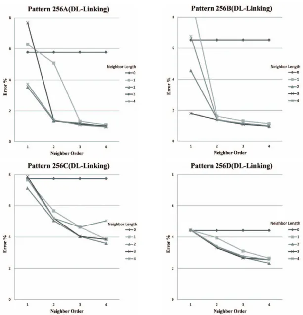
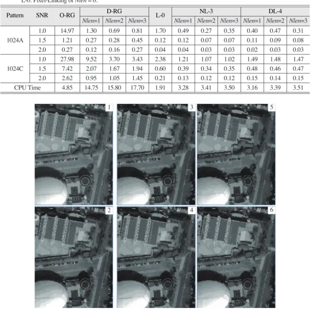
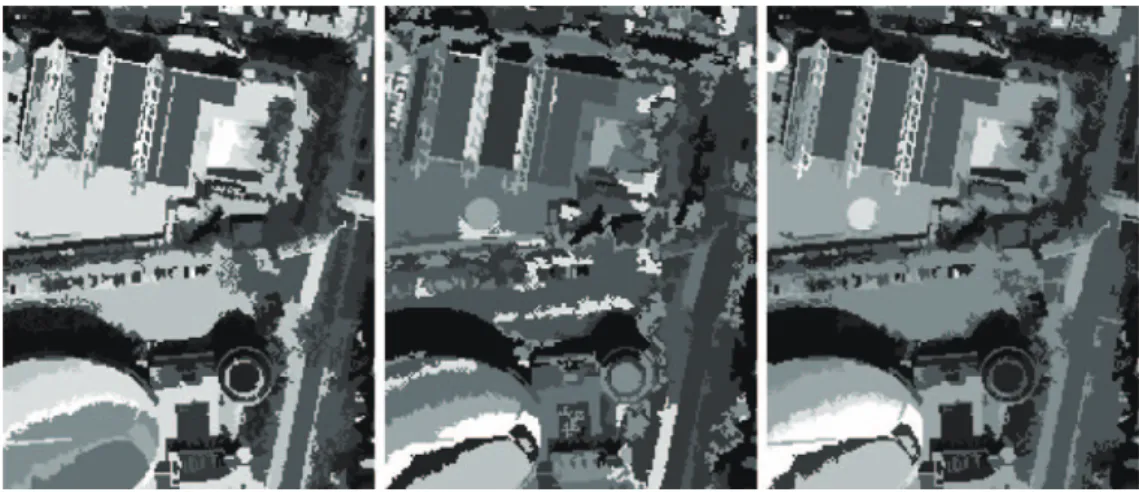
Abstract : An efficient method for the unsupervised classification of high resolution imagery is suggested in this paper. It employs pixel-linking and merging based on the adjacency graph. The proposed algorithm uses the neighbor lines of 8 directions to include information in spatial proximity. Two approaches are suggested to employ neighbor lines in the linking. One is to compute the dissimilarity measure for the pixel-linking using information from the best lines with the smallest non. The other is to select the best directions for the dissimilarity measure by comparing the non-homogeneity of each line in the same direction of two adjacent pixels. The resultant partition of pixel-linking is segmented and classified by the merging based on the regional and spectral adjacency graphs. This study performed extensive experiments using simulation data and a real high resolution data of IKONOS. The experimental results show that the new approach proposed in this study is quite effective to provide segments of high quality for object-based analysis and proper land-cover map for high resolution imagery of urban area.

Key Words : Image segmentation, Image classification, Unsupervised analysis, Pixel-linking, High resolution imagery, Regional adjacency graph, Spectral adjacency graph

Received November 12, 2011; Revised December 14, 2011; Accepted December 15, 2011.

†

Corresponding Author: Sang-Hoon Lee ([email protected])

prerequisite of object-based analysis is image segmentation which is the process of partitioning an image into non-intersecting regions such that each region is homogeneous and the union of any two adjacent regions is not homogeneous (Fu and Mui, 1981; Pal and Pal, 1993).

Image segmentation algorithms can be divided into four methods (Cheng et al., 2001): 1) histogram thresholding, 2) image feature-space clustering, 3) region-based, and 4) edge-based. The histogram thresholding method is a simple and widely used technique for segmenting monochrome images (Mao and Jain, 1992; Hofmann et al., 1998). An image is segmented using several threshold values selected through image histogram inspection either manually or automatically. The image feature-space clustering method is a multi-dimensional extension of the concept of histogram thresholding, and it segments an image by grouping similar vectors (pixels) into one segment (Hall et al., 1992). Image clustering and histogram thresholding methods have disadvantages, including the fact that they do not incorporate the spatial characteristics of image data. On the other hand, region-based image segmentation approaches, including region growing, region splitting, region merging, or their combinations, group spatially connected pixels into homogeneous segments. The major advantage of the region-based methods is that segments are guaranteed to be homogeneous spatially. Image segments can also be obtained through the detection of edges associated with regions. An edge-based segmentation first detects edges within an image, and then applies additional steps to produce a closed curve or boundary to complete the segment (Haralick and Shapiro, 1985;

Cheng et al., 2001; Shih and Cheng, 2005).

Lee (2006a) suggested a regional growing segmentation based on regional adjacency graph (RAG) (Pavlidis, 1980), which merges spatially

adjacent regions and then generates an image partition such that no union of any neighboring segments is uniform. Another region merging technique based on the RAG was suggested for the segmentation of high-spatial resolution imagery (Lee, 2010). This algorithm used directional neighbor-line average feature vectors to improve the quality of segmentation. The feature vector consists of 9 components which includes an observation and 8 directional averages. This study proposes an efficient unsupervised classification for high-spatial resolution imagery. The proposed algorithm is a multistage scheme including pixel-linking, RAG-based merging and SAG-based merging. The spectral adjacency graph (SAG) represents the structure of spectral adjacency in remote sensing imagery, while the RAG describes spatial contiguity. The SAG-based merging is a classification process on the regions resulted from image segmentation (Lee, 2006b).

2. Pixel-linking

The first stage is a process to link every pixel in the image with one of 8 neighbor pixels. Consider the (i, j)th pixel with a neighbor index set of 8 pixels, R(i, j) = {(i, j + 1), (i + 1, j), (i + 1, j + 1), (i + 1, j _ 1)

(i, j _ 1), (i _ 1), j _ 1), (i _ 1, j + 1)}.

The closest neighbor (CN) of pixel (i, j) is defined as

CN(i, j) = argmin

d[(i, j), (r, s)] (1) where d[(i, j), (r, s)] is the dissimilarity measure between pixels (i, j) and (r, s). The linking procedure is to find the closest neighbor and connect two pixels.

Fig. 1 displays an example of the pixel linking. In the left figure, the arrows indicate the CN of each pixel:

for the first and second rows,

CN(1, 1) = (2, 2) CN(1, 2) = (2, 3) CN(1, 3) = (2, 3) CN(2, 1) = (2, 2) CN(2, 2) = (1, 1) CN(2, 3) = (1, 3) CN(1, 4) = (1, 5) CN(1, 5) = (1, 4)

CN(2, 4) = (2, 3) CN(2, 5) = (3, 5)

After connecting the pixels, the image is partitioned as 7 segments as shown in the right figure.

The pair of pixels is defined as the mutual closest neighbor (MCN) iff CN(i, j) = (r, s) and CN(r, s) = (i, j).

The pixels (1, 1) and (2, 2) are an MCN pair. In the segmentation resulted from the linking, each segment must have only one MCN pair.

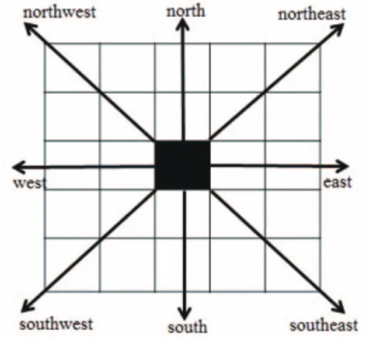
In this study, the dissimilarity measure is chosen to include neighbor information in spatial proximity. The neighbor lines of 8 directions are defined as a set of pixel indexes: given the length of neighbor line, Nlen,

NL

(i, j) = {NL

(i, j), dir}

dir = east, south, southeast, southwest, west, north, northwest, northeast

NL

(i, j) = {(i, j + k), k = 1, , Nlen}

NL

(i, j) = {(i + k, j), k = 1, , Nlen}

NL

(i, j) = {(i + k, j + k), k = 1, , Nlen}

NL

(i, j) = {(i + k, j _ k), k = 1, , Nlen}

NL

(i, j) = {(i, j _ k), k = 1, , Nlen}

NL

(i, j) = {(i _ k, j), k = 1, , Nlen}

NL

(i, j) = {(i _ k, j _ k), k = 1, , Nlen}

NL

(i, j) = {(i _ k, j + k), k = 1, , Nlen}

Fig. 2 shows the neighbor lines of Nlen = 2. Given an order of directional selection, Nord,

d[(i, j), (r, s)] = Q(R)

R = {(i, j), (r, s), NL

(i, j), , NL

(i, j), NL

(r, s), , NL

(r, s),}

(2)

where Q is a non-homogeneity measure of the pixels corresponding to the index set R, and NL

(i, j) is the NL

(i, j) of Q which is the kth smallest among {Q((i, j), NL

(i, j)), dir/dir(i, j)(r, s)} where represents the direction of (i, j) toward (r, s) and

dir/dir(i, j)(r, s) means the exclusion of dir(i, j)(r, s) from dir. For example, the measure of pixels (i, j) and (i, j + 1) excludes NL

(i, j) and NL

(i, j + 1). The internal variation is used as Q:

Q(R) = (3)

_ x =

where n

is the number of pixel indexes of R.

Fig. 4 shows the results of pixel-linking with Nord

= 0, 1, and 2 and Nlen = 2 respectively. The linking of Nord = 0 had three pixels (dotted) which are

x

n

(x

_ _x)

(x

_ _x) n

Fig. 1. Example of pixel-linking.

Fig. 2. Neighbor lines of Nlen = 2.

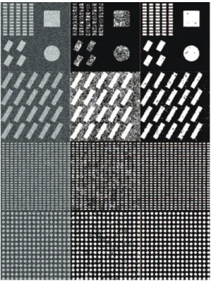
Fig. 3. Simulation image of 9 9 with 3 classes.

S

(i, j) R

S

(i, j) R

wrongly partitioned, and one pixel is connected to the pixels of different class when using Nord = 1. The results show the pixel-linking with neighbor lines has the potentiality for the improvement of boundary configuration in image segmentation.

Another approach is also proposed in order to include directional neighbor information in the pixel- linking. It is a very similar idea with the segmentation using directional features suggested in Lee (2010).

The dissimilarity measure is defined :

d[(i, j), (r, s)] = Q

((i, j), (r, s)) (4) where

Q

((i, j), (r, s)) = Q((i, j), NL

(i, j), NL

(r, s), Q

((i, j), (r, s)) = Q((i, j), NL

(i, j), NL

(r, s), Q

((i, j), (r, s)) is the kth smallest Q among {Q((i, j)), {Q

((i, j), (r, s)), dir/dirLO}, Q

((i, j), (r, s))}, dirL

= dir(i, j)(r, s), dirO = dir(r, s) and dirLO = {dirL, dirO}. The scheme of Eq. (1) is called as NL-Linking and the other of Eq. (3) as DL-Linking.

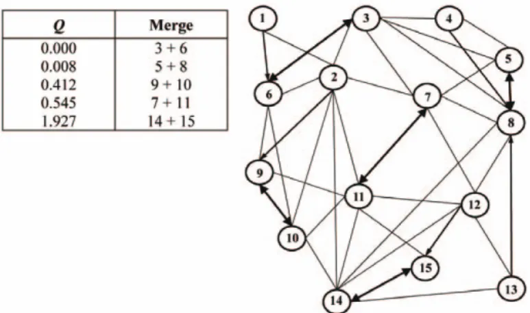
3. RAG- and SAG- Based MCN Merging

The computational efficiency of region merging is mainly dependent on how to find the best pair to be merged. Let that R

is the index set of neighborhood regions of region j. The closest neighbor of region j is

defined as

CN(j) = arg min

d(j, k)

where d(j, k) is the dissimilarity measure between regions j and k, and R

is the index set of regions considered to be merged with region j. In the adjacency graph, each region is represented by a graph node and there exists the edge between two nodes if the corresponding regions are neighboring. A merging cost is assigned to each edge as dissimilarity measure between two neighboring regions. The algorithm based on the adjacency graph merges the regions connected by the edge with the minimum cost, which must be a MCN. For the edge cost, the RAG-based merging uses the non-homogeneity measure of EQ. (2) and the SAG-based merging the simple Euclidian distance :

d(j, k) = Q(R

, R

) = ( _ x

_ _

x

)

( _ x

_ _

x

)

_ x = (5)

Lee (2006a) used a data structure of Min-Heap (van Wyk, 1988) for a MCN-based image classification to search the best pair in the present set of MCN pairs, that is, to find the edge with the minimum cost in the adjacency graph. The proposed algorithm continues to search a pair to be merged with a Min- Heap structure and update the adjacency graph

x

n

Nord

S

k=1

Fig. 4. Pixel-linking results of simulation image in Fig. 3 using Nord = 0, 1, and 2 (from left) with Nlen = 2.

S

(i, j) R

according to merging at each iteration and stops the iteration for a given condition. It is difficult to define an appropriate measure of homogeneity to establish a

rule for the optimal number of regions in segmentation. The model fitting approaches using information criteria which measure the trade-off Fig. 5. RAG and MCN pairs of 15 segments resulted from NL-Linking of Nlen = 2 and Nord = 2 for simulation image in Fig. 3.

Fig. 6. Image Partition, RAG and MCN pairs of 14 segments resulted from RAG-based merging for simulation image in Fig. 3.

Fig.7. Image Partition and RAG of 7 segments from RAG-based merging for simulation image in Fig. 3.

between the likelihood and the penalty for increasing the model’s order have been applied for cluster validation in image analysis (Won and Derin, 1992).

The Lee’s region-growing segmentation procedures (Lee, 2004, 2006a) use the criterion of selecting the optimal state that maximizes Schwarz’s information criterion (Schwarz, 1978).

Fig. 5 shows the RAG of the third partition in Fig.

4 resulted from NL-Linking with Nlen = 2 and Nord

= 2. In the RAG, the arrow represents the CN and the MCNs have a bidirectional arrow. The table in the figure contains the Q values of the MCNs. The update of RAG shows in Fig. 6 after merging the best pair of node 3 and node 6. The RAG-based merging produced the image segmentation of 7 regions for a given criterion as shown in Fig.7. Fig. 8 gives an example of SAG. Table 1 shows the Q values when merging two regions in the resultant partition of 7 segments each other. If the threshold for spectral neighborhood is 21.97, the SAG and MCN pairs of the 7 segments are illustrated in figure.

4. Experiments

The proposed method was first evaluated using simulation data generated by the Monte Carlo method. The gray-scaled simulation images were generated using diverse patterns by adding white Gaussian noise. In order to represent varying noise levels in the simulation images, the signal-to-noise ratio (SNR) is defined as the ratio of the smallest intensity-level difference to the average noise standard deviation. For computational convenience, the simulation used an identical variance of all region-classes and a constant difference between contiguous magnitude levels in mean intensity for the same pattern.

The first simulation experiment evaluated the performance of the linking algorithm for various neighbor lengths and orders. The simulation data of SNR = 3.0 were generated from four binary patterns of 256 256 displayed in Fig. 8, and classified with the proposed method using the pixel-linking of Nlen

= 0, 1, 2, 3, 4 and Nord = 1, 2, 3, 4. Figs. 9 and 10 Table 1. Q Values when merging two of 7 segments each other.

ID JD Q

2 20.837

3 1188.254

4 151.660

5 161.790

6 1283.272

7 474.919

3 531.434

4 50.640

2 5 90.766

6 595.983

7 149.115

4 170.632

5 12.618

6 3.822

7 207.236

5 20.409

4 6 208.517

7 7.747

5 6 20.491

7 10.295

6 7 261.766

ID JD Q

Fig. 8. Four binary pattern of 256 256

displays the classification errors in percentage resulted from NL-Linking and DL-Linking respectively. The NL-Linking produced very fine results for patterns 256A and 256B including large- scale features regardless of Nlen and Nord, while the DL-Linking is not working well with Nlen = 1. For the patterns with small-scale features, the performance of both methods is not good as for the large scale ones. For pattern 256C, the NL-Linking of

Nlen = 4 showed that the error increases as the Nord becomes larger. It implies that a big Nlen is not appropriate for small-sclae features. Fig. 11 illustrated the examples of classified images resulted from the linking without neighbor lines and the NL-Linking of Nlen = 2 and Nord, = 3. These results suggest using Nlen = 2 and that the DL-Linking would have better result with a larger Nord. The NL-Linking of Nlen = 2 shows good performance for all values of Nord.

Fig. 9. Classification errors in percentage when using NL-Linking .

The next simulation experiment used four patterns with different number of classes as shown in Fig. 12.

Table 2 contains the classification errors in percentage for single band simulation images of SNR

= 3. 0 and 4.0 when using NL-Linking of Nord = 3 and DL-Linking of Nord = 4. Except the cases of Nlen = 1, the NL-Linking showed better performance than the DL-Lining, and more better for the higher noisy data. To compare the new method to the

previous RAG-based merging (Lee, 2010), the three band simulation data were generated for pattern 1024A and1024C. Table 3 compared in classification error for simulation data of SNR = 1.0, 1.5, and 2.0.

The performance of the new method was substantially better. Especially, the computational efficiency considerable increased in the proposed scheme.

The methodology was next applied to IKONOS

Fig. 10. Classification errors in percentage when using DL-Linking .

data acquired from the north area of Anyang city, Korea as in (Lee, 2010), using the pixel-linking of Nlen = 0, 1, 2, 3, 4 and Nord = 1, 2, 3, 4. When using Nlen = 3, 4 and Nord = 3, 4, image segmentation of the proposed scheme failed in figure out very detailed structures on the ground such as the line of one pixel width. Though Nlen = 0 and Nlen = 1 with Nord = 1, 2 succeeded in finding the complicate structures, the large structures were partitioned into several segments. Fig. 13 shows the results of image segmentation using Nlen = 0 and NL-Linking and DL-Linking of Nlen = 2 and Nord = 1, 2. The figure displays a sub-area of the whole image. As shown in this figure, the DL-Linking of Nlen = 2 and Nord = 1 produced the best segmentation. Fig. 14 shows the classified images of Nlen = 0 and NL-Linking and DL-Linking of Nlen = 2 and Nord = 1. The linking of Nlen = 0 failed in correctly segmenting the large rectangle structure in top left corner.

Fig. 12. Patterns similar to natural scene.

Fig. 11. Examples of Simulation images of SNR = 3.0 from 4 patterns and class maps produced when using Linking without neighbor lines (center) and NL-Linking with Nlen = 2 and Nord = 3 (right).

NL-3 DL-4 NL-3 DL-4

0 15.79 5.62

1 15.60 14.71 0.07 0.06

1024A 2 1.23 7.65 0.04 0.05

3 0.16 4.87 0.04 0.05

4 0.14 4.13 0.05 0.05

0 37.16 1.77

1 12.87 5.65 0.69 0.66

1024B 2 1.88 3.37 0.43 0.50

3 1.45 3.01 0.39 0.50

4 1.35 3.02 0.38 0.50

0 35.65 0.17

1 35.51 32.84 0.10 0.10

1024C 2 0.31 0.52 0.07 0.08

3 0.23 0.46 0.06 0.08

4 0.22 0.43 0.06 0.08

0 36.13 0.56

1 34.28 5.09 0.29 0.28

1024D 2 0.79 1.36 0.18 0.22

3 0.62 1.18 0.17 0.23

4 0.58 1.21 0.17 0.24

NL-3 DL-4 NL-3 DL-4

5. Conclusion

This paper extended and improved a RAG-based MCN merging for image segmentation. The quality of segmentation results directly affects the accuracy

of the subsequent image classification. The pixel- linking was proposed as a preprocessor of RAG- based MCN merging by connecting each pixel with one of its neighbors. The simulation experiment showed that the pixel-linking performs in Table 3. Comparison of classification errors in percentage for 3 band simulation images of SNR = 1.0, 1.5 and 2.0 when using

different RAG-based image segmentation:

O-RG: original RAG-based segmentation

D-RG: RAG-based segmentation with 8 directional features L-0: Pixel-Linking of Nlen = 0.

Pattern SNR O-RG D-RG L-0 NL-3 DL-4

Nlen=1 Nlen=2 Nlen=3 Nlen=1 Nlen=2 Nlen=3 Nlen=1 Nlen=2 Nlen=3 1.0 14.97 1.30 0.69 0.81 1.70 0.49 0.27 0.35 0.40 0.47 0.31 1024A 1.5 1.21 0.27 0.28 0.45 0.12 0.12 0.07 0.07 0.11 0.09 0.08 2.0 0.27 0.12 0.16 0.27 0.04 0.04 0.03 0.03 0.02 0.03 0.03 1.0 27.98 9.52 3.70 3.43 2.38 1.21 1.07 1.02 1.49 1.48 1.47 1024C 1.5 7.42 2.07 1.67 1.94 0.60 0.39 0.34 0.35 0.48 0.46 0.47 2.0 2.62 0.95 1.05 1.45 0.21 0.13 0.12 0.12 0.15 0.14 0.15 CPU Time 4.85 14.75 15.80 17.70 1.91 3.28 3.41 3.50 3.16 3.39 3.51

Pattern SNR O-RG D-RG

L-0 NL-3 DL-4

Nlen=1 Nlen=2 Nlen=3 Nlen=1 Nlen=2 Nlen=3 Nlen=1 Nlen=2 Nlen=3

Fig. 13. Segmentation images of sub-area IKONOS panchromatic image acquired from north area of Anyang city, Korea using pixel- linking and RAG-based MCN merging: (1) Observation, (2) Nlen = 0, (3) NL-Linking with Nlen = 2 and Nord = 1, (4) DL- Linking with Nlen = 2 and Nord = 1, (5) NL-Linking with Nlen = 2 and Nord = 2, (6) NL-Linking with Nlen = 2 and Nord = 1.

2

1 3

4

5

6

classification accuracy and computational efficiency considerably better than the original RAG-based merging. The proposed method is designed to use 8 neighbor lines in order to include neighbor information in spatial proximity in the linking, and employed two approaches, NL-Linking and DL- Linking. In the NL-Linking, the dissimilarity measure for the best connection is computed with a given number of 8 neighbor lines which have the smallest non-homogeneity. DL-Linking computes the dissimilarity measure by combining a given number of the smallest directional non-homogeneity measures. The directional measure is computed with the neighbor lines of same direction in a pair of two neighboring pixels. Both of the linking schemes substantially performed better with the neighbor lines.

In the simulation experiment, the NL-Linking generally showed better performance than the DL- Linking for classification error. However, for real remote sensing data, the DL-Linking somewhat produced image segmentation which better displays a very detailed structure. It is more important to use appropriate length and order of neighbor lines in order to correctly figure out multi-scale features in urban environment.

The extensive experiments indicate that the

proposed method using the pixel-linking is exceptionally capable of providing the segments of high quality for successful object-based image analysis in remote sensing applications.

Acknowledgment

This research was supported by a by KRF-D01078 grant.

References

Blaschke, T. 2005. A Framework for Change Detection Based on Image Objects, In: S.

Erasmi, B. Cyffka, and M. Kappas, Editors, G?ttinger Geographische Abhandlungen, Göttingen, 113:1?9.

Blaschke, T., 2009. Object based image analysis for remote sensing, ISPRS Journal of Photogrammetry and Remote Sensing 65: 2-16.

Cheng, H. D. , X. H. Jiang, Y. Sun, and J. L. Wang, 2001. Color image segmentation: advances and prospects, Pattern Recognition, 34: 2259- 2281.

Fig. 14. Classified images of (2), (3) and (4) in Fig. 4 using SAG-based MCN merging.

Fu, K. S. and J. K. Mui, 1981. A survey on image segmentation, Pattern Recognition, 13:3-16.

Hall, L. O., A. M. Bensaid, L. P. Clarke, R. P.

Velthuizen, M. S. Silbiger, and J. C. Bezdek, 1992. A comparison of neural network and fuzzy clustering techniques in segmenting magnetic resonance images of the brain, IEEE Transactions on Neural Networks, 3: 672- 681.

Haralick, R. M. and L. G. Shapiro, 1985. Survey of image segmentation techniques, Computer Vision Graphics Image Process, 29:100-132.

Hofmann, T., J. Puzicha, and J. Buhmann, 1998.

Unsupervised texture segmentation in a deterministic annealing framework, IEEE Transactions on Pattern Analysis and Machine Intelligence, 20: 803-818.

Lee, S-H., 2004. Unsupervised Image Classification using Region-growing Segmentation based on CN-chain, Korean Journal Remote Sensing, 20: 215-225.

Lee, S-H., 2006a. RAG-based Image Segmentation using Multiple Windows, Korean Journal Remote Sensing, 22: 601-612 (in Korean).

Lee, S-H., 2006b. RAG-based Hierarchical Classification, Korean Journal Remote

Sensing, 22: 613-619 (in Korean).

Lee, S-H., 2010. Region Growing Segmentation with Directional Features, Korean Journal Remote Sensing, 26: 731-740.

Jensen, J. R., 2005. Introductory Digital Image Processing: a Remote Sensing Perspective (third ed.), Prentice-Hall, Upper Saddle River.

Mao, J. and A. Jain, Texture classification and segmentation using multiresolution simultaneous autoregressive models, Pattern Recognition, 25 :173-188

Pal, N. R. and S. K. Pal, 1993. A review on image segmentation techniques, Pattern Recognition, 26: 1277-1294.

Shih F. Y. and S. Cheng, 2005. Automatic seeded region growing for color image segmentation, Image and Vision Computing, 23: 877-886.

Pavlidis, T., 1980. Structural Pattern Recognition, New York: Springer.

vanWyk, C., 1988. Data Structures and C Programs.

Reading, MA: Addison-Wesley.

Won, C. S. and H. Derin, 1992.Unsupervised segmentation of noisy and textured images using Markov random fields, CVGIP, 54:

308-328.