2005, Vol. 16, No. 4, pp. 1067∼1078
Bayesian Analysis for the Difference of Exponential Means
Sang Gil Kang
1)⋅ Dal Ho Kim
2)⋅ Woo Dong Lee
3)Abstract
In this paper, we develop the noninformative priors for the exponential models when the parameter of interest is the difference of two means. We develop the first and second order matching priors. We reveal that the second order matching priors do not exist. It turns out that Jeffreys' prior does not satisfy the first order matching criterion. The Bayesian credible intervals based on the first order matching meet the frequentist target coverage probabilities much better than the frequentist intervals of Jeffreys' prior.
Keywords : Difference of Two Means, Exponential Distributions, Jeffreys' Prior, Matching Prior
1. Introduction
The exponential distribution plays an important role in the field of reliability.
The reasons for using the exponential distribution in reliability applications can be found in the early work of Davis (1952), Epstein and Sobel (1953), and others.
Further justification, in the form of theoretical arguments to support the use of the exponential distribution as the failure law of complex equipment, is presented in the book by Barlow and Proschan (1975) and Lawless (2003).
The present paper focuses on noninformative priors for the difference of two exponential means. We consider Bayesian priors such that the resulting credible intervals for the difference of two exponential means have coverage probabilities 1) First Author : Department of Applied Statistics, Sangji University, Wonju, 220-712,
Korea
E-mail : [email protected]
2) Department of Statistics, Kyungpook National University, Taegu, 702-701, Korea
3) Corresponding Author : Department of Asset Management, Daegu Hanny University, Kyungsan, 712-715, Korea
E-6mail : [email protected]
equivalent to their frequentist counterparts. Although this matching can be justified only asymptotically, our simulation results indicate that this is indeed achieved for small or moderate sample sizes as well.
This matching idea goes back to Welch and Peers (1963). Interest in such priors revived with the work of Stein (1985) and Tibshirani (1989). Among others, we may cite the work of Mukerjee and Dey (1993), DiCiccio and Stern (1994), Datta and Ghosh (1995a,b, 1996), Mukerjee and Ghosh (1997) and Sang Gil Kang (2004).
On the other hand, Ghosh and Mukerjee (1992), and Berger and Bernardo (1989,1992) extended Bernardo's (1979) reference prior approach, giving a general algorithm to derive a reference prior by splitting the parameters into several groups according to their order of inferential importance. This approach is very successful in various practical problems. Quite often reference priors satisfy the matching criterion described earlier.
The problem of comparison for two exponential means has been investigated by many authors. For the comparison of two exponential distributions, most of the studies are the ratio of means. However there is a little work in the interval estimation for the difference between two exponential means.
Akahira (2002) proposed a systematic method for the construction of a confidence interval for the difference between two means in the exponential distributions. But the proposed method can only apply for the case of equal sample sizes (balanced case). And to find the interval, for a given significance level and sample size, a function satisfying some condition must always be computed with respect to the level and sample size, and even the function may not be unique.
Since there is little work to this problem in Bayesian framework and we want to find a Bayesian solution of this problem which can cover unbalance case.
The outline of the remaining sections is as follows. In Section 2, we develop probability matching priors for the difference of two exponential means. We reveal that the second order matching prior does not exist. It turns out that the Jeffreys' prior does not satisfy a first order matching criterion. And we provide the propriety of the posterior distribution for the first order matching priors in Section 3. In Section 4, simulated frequentist coverage probabilities under the proposed priors are given.
2. The Noninformative Priors
For a prior
π
, letθ
11−α(π;Y)
denote the(1 − α )
th percentile of the posterior distribution ofθ
1, that is,Pπ
[θ
1≤θ
11− α(π;Y)│Y] = 1 − α,
where
θ = (θ
1, , θt)
T andθ
1 is the parameter of interest. We want to find priorsπ
for whichP [θ
1≤θ
11−α(π;Y)│θ ] = 1 − α + o (n
−u).
(1) for some u > 0, as n goes to infinity. Priorsπ
satisfying (1) are called matching priors. If u = 1/2, thenπ
is referred to as a first order matching prior, while if u = 1,π
is referred to as a second order matching prior.Consider that
X
1, , X
n1 are independent and identically distributed random variables according to the exponential distribution with meanµ
1 andY
1, , Y
n2
are independent and identically distributed random variables according to the exponential distribution with mean
µ
2. Then the likelihood function of μ1 and μ2is
L (µ1, µ2
)∝
1 µ
1n1
1 µ
2n2
e xp
− Σi = 1
n1 x
i
µ
1− Σi = 1
n2
y
iµ
2 , (2) where theµ
1> 0
and theµ
2> 0.
In order to find matching priors
π
, letθ
1= µ
1− µ
2 andθ
2=
n1µ
1+
n2µ
2.With the above parametrization, the likelihood function of parameters
(θ
1, θ
2)
is given byL(θ
1, θ
2) ∝ θ
n21+ n2n
1+ n
2+ θ
1θ
2+ [(n
2− n
1+ θ
1θ
2)
2+ 4n
1n
2]
1/2 −n1n
1+ n
2− θ
1θ
2+ [(n
2− n
1+ θ
1θ
2)
2+ 4n
1n
2]
1/2 −n2e xp
− Σi = 1
n1
2θ
2x
in
1+ n
2+ θ
1θ
2+ [(n
2− n
1+ θ
1θ
2)
2+ 4n
1n
2]
1/2−
Σ
i = 1
n2
2θ
2y
in
1+ n
2− θ
1θ
2+ [(n
2− n
1+ θ
1θ
2)
2+ 4n
1n
2]
1/2.
(3)
Based on (3), the Fisher information matrix is given by
I =
I
110
0 I
22 ,where
I
11= 8n
1n
2θ
22[(n
1+ n
2)g (θ
1, θ
2)
1/2+ (n
1+ n
2)
2+ (n
2− n
1)θ
1θ
2]
g (θ
1, θ
2)
1/2[n
1+ n
2− θ
1θ
2+ g (θ
1, θ
2)
1/2]
2[n
1+ n
2+ θ
1θ
2+ g (θ
1, θ
2)
1/2]
2,I
22= 2 [(n
1+ n
2)
2+ (n
2− n
1)θ
1θ
2+ (n
1+ n
2)g (θ
1, θ
2)
1/2]
3θ
22g (θ
1, θ
2)
1/2[n
1+ n
2− θ
1θ
2+ g (θ
1, θ
2)
1/2]
2[n
1+ n
2+ θ
1θ
2+ g (θ
1, θ
2)
1/2]
2and
g (θ1, θ2
) = (n
2−
n1+ θ
1θ
2)
2+ 4n
1n2.From the above Fisher information matrix I, one can verify that
θ
1 is orthogonal toθ
2 in the sense of Cox and Reid (1987). Following Tibshirani (1989), the class of first order probability matching prior is characterized byπ
(1)m(θ
1, θ
2)
∝ θ
2[(n
1+ n
2)g (θ
1, θ2)
1/2+ (n
1+ n
2)
2+ (n
2−
n1)θ
1θ
2]
1 2
g (θ1, θ2
)
1/4[n
1+ n
2− θ
1θ
2+ g (θ
1, θ2)
1/2][n
1+ n
2+ θ
1θ
2+ g (θ
1, θ2)
1/2]
d (θ2),
(4) whered (θ
2) > 0
is an arbitrary function differentiable in its argument.According to Mukerjee and Ghosh (1997), the class of prior given in (4) can be narrowed down to the second order probability matching priors.
A second order probability matching prior is of the form (4), and also d must satisfy an additional differential equation (cf (2.10)) of Mukerjee and Ghosh (1997), namely
1
6
d (θ2) ∂
∂θ
1I−3 2
11 L1, 1, 1
+ ∂
∂θ
2I−1 2
11 L112I22d (θ2
) = 0,
(5) whereL1, 1, 1
= E
∂l ogL
∂θ
13
= h
1(θ
1, θ
2)
g (θ
1, θ
2)
3/2(n
1+ n
2− θ
1θ
2+ g (θ
1, θ
2)
1/2)
6(n
1+ n
2+ θ
1θ
2+ g (θ
1, θ
2)
1/2)
6,
L
112= E ∂
3l ogL
∂θ
21∂θ
2
= h
2(θ
1, θ
2)
g (θ
1, θ
2)(n
1+ n
2− θ
1θ
2+ g (θ
1, θ
2)
1/2)
3(n
1+ n
2+ θ
1θ
2+ g (θ
1, θ
2)
1/2)
3,
.h
1(θ
1, θ
2) = − 512n
1n
2θ
32[(n
1+ n
2)
2+ (n
2− n
1)θ
1θ
2+ (n
1+ n
2)g (θ
1, θ
2)
1/2]
3(n
1− n
2)(n
1+ n
2)
4− θ
1θ
2[3 (n
1+ n
2)
2(n
12− n
1n
2+ n
22)
+ 3 (n
23− n
13)θ
1θ
2+ (n
22+ n
12)θ
21θ
22] + (n
1+ n
2)[(n
1− n
2)(n
1+ n
2)
2− (2n
12− n
1n
2+ 2n
22)θ
1θ
2+ (n
1− n
2)θ
21θ
22]g (θ
1, θ
2)
1/2and
h
2(θ
1, θ
2) = − 64n
1n
2(n
1+ n
2)θ
2[(n
1+ n
2)
4+ 2 (n
2− n
1)(n
1+ n
2)
2θ
1θ
2+ (n
12− n
1n
2+ n
22)θ
21θ
22] − 64n
1n
2θ
2[(n
1+ n
2)
4
+ 2 (n
2− n
1)(n
1+ n
2)
2θ
1θ
2+ (n
12+ n
1n
2+ n
22)θ
21θ
22]g (θ
1, θ
2)
1/2. Then (5) simplifies to1
6
d (θ2) ∂
∂θ
1 w1(θ
1, θ2) + ∂
∂θ
2 w2(θ
1, θ2)d (θ
2) = 0,
(6) where
w
1(θ
1, θ
2)
= (8n
1n
2)
− 3/2θ
− 32h
1(θ
1, θ
2)[(n
1+ n
2)g
1/2+ (n
1+ n
2)
2+ (n
2− n
1)θ
1θ
2]
− 3/2g (θ
1, θ
2)
3/4(n
1+ n
2− θ
1θ
2+ g (θ
1, θ
2)
1/2)
3(n
1+ n
2+ θ
1θ
2+ g (θ
1, θ
2)
1/2)
3 andw
2(θ
1, θ
2) = (8n
1n
2)
− 1/2θ
2h
2(θ
1, θ
2)
2g (θ
1, θ
2)
1/4[(n
1+ n
2)g
1/2+ (n
1+ n
2)
2+ (n
2− n
1)θ
1θ
2]
7/2 . However there can be no solution to (6) unless the d is the function ofθ
1 andθ
2. Thus the second order matching prior does not exist.From the Fish information matrix I, the Jeffreys' prior is given by
π
J(θ
1, θ
2)
∝ [(n
1+ n
2)g (θ
1, θ
2)
1/2+ (n
1+ n
2)
2+ (n
2− n
1)θ
1θ
2]
2g (θ
1, θ
2)
1/2[n
1+ n
2− θ
1θ
2+ g (θ
1, θ
2)
1/2]
2[n
1+ n
2+ θ
1θ
2+ g (θ
1, θ
2)
1/2]
2.
(7) Remark 1. In the original parameterization(µ
1, µ
2)
, the first order matching prior is given byπ
(1)m(µ
1, µ
2)∝µ
− 11µ
− 12
n
1µ
21+ n
2µ
221/2
d (θ
2(µ
1, µ
2)).
And the Jeffreys' prior is given by
π
J(µ
1, µ
2)∝µ
− 11µ
− 12.
(8) Note that the matching priors (4) include many different matching priors because of the arbitrary selection of the function d. However every function is not permissible in the construction of priors. For instance, we can consider any function of the formθ
− a2 . If a is negative integer, then the posterior distribution under function of the formθ
− a2 is proper. But the condition of propriety in this form strongly depend on the a. Moreover the posterior under this form is complex. Also there does not seem to be any improvement in the coverage probabilities with this posterior distribution. So we have chosen d to be a constant function. The resulting prior is given byπ
(1)m(θ
1, θ
2)
∝ θ
2[(n
1+ n
2)g (θ
1, θ
2)
1/2+ (n
1+ n
2)
2+ (n
2− n
1)θ
1θ
2]
1/2g (θ
1, θ
2)
1/4[n
1+ n
2− θ
1θ
2+ g (θ
1, θ
2)
1/2][n
1+ n
2+ θ
1θ
2+ g (θ
1, θ
2)
1/2] .
(9) Thus in the original parameterization(µ
1, µ
2)
, the first order matching prior is given byπ
(1)m(µ
1, µ
2)∝µ
− 11µ
− 12
n
1µ
21+ n
2µ
221/2
.
(10)3. Implementation of the Bayesian Procedure
We investigate the propriety of posteriors for a general priors which include Jeffreys' prior (8) and the first order matching prior (10). We consider the class of priors
π
g(µ
1, µ
2)∝µ
− a1µ
− b2
n
1µ
21+ n
2µ
22c
,
(11)where a > 0, b > 0 and c≥0. The following theorem can be proved.
Theorem 1. The posterior distribution of
(µ
1, µ
2)
under the prior (11) is properif
n
1+ a − 1 > 0
andn
2+ b − 1 > 0
.Proof. Under the prior (11), the joint posterior for
µ
1 andµ
2 given x and y isπ (µ
1, µ
2│x, y)∝
1 µ
1n1+ a
1 µ
2n2+ b
n
1µ
21+ n
2µ
22c
e xp
− Σ
i = 1 n1
x
iµ
1− Σ
i = 1 n2
y
iµ
2 . For1≤µ
1< ∞
and1≤µ
2< ∞
,
1
∞ 1
∞
π (µ1, µ2│ x, y )d µ1d µ2
≤
1
∞ 1
∞
1 µ
1n1+ a
1 µ
2n2+ b
(
n1+ n
2)
ce xp
− Σ
i = 1 n1
x
iµ
1− Σ
i = 1 n2
y
iµ
2dµ
1dµ
2≤
0
∞ 0
∞
1 µ
1n1+ a
1 µ
2n2+ b
(
n1+ n
2)
ce xp
− Σ
i = 1 n1
x
iµ
1− Σ
i = 1n2
y
iµ
2dµ
1dµ
2< ∞
, ifn
1+ a − 1 > 0
andn
2+ b − 1 > 0
. For0 < µ
1< 1
and1≤µ
2< ∞
,
1
∞ 0
1
π (µ1, µ2│ x, y )d µ1d µ2
≤
1
∞ 0
1
1 µ
1n1+ a + 2c
1 µ
2n2+ b
(
n1+ n
2)
ce xp
− Σ
i = 1 n1
x
iµ
1− Σ
i = 1 n2
y
iµ
2dµ
1dµ
2≤
0
∞ 0
∞
1 µ
1n1+ a + 2c
1 µ
2n2+ b
(
n1+ n
2)
ce xp
− Σ
i = 1 n1
x
iµ
1− Σ
i = 1 n2
y
iµ
2dµ
1dµ
2< ∞
,if
n
1+ a + 2c − 1 > 0
andn
2+ b − 1 > 0
. For0 < µ
1< 1
and0 < µ
2< 1
,
0 1
0 1
π ( µ1, µ2│ x, y )d µ1d µ2
≤
0 1
0 1
1 µ
1n1+ a + 2c
1 µ
2n2+ b + 2c
(
n1+ n
2)
ce xp
− Σ
i = 1 n1
x
iµ
1− Σ
i = 1n2
y
iµ
2dµ
1dµ
2≤
0
∞ 0
∞
1 µ
1n1+ a + 2c
1 µ
2n2+ b + 2c
(
n1+ n
2)
ce xp
− Σ
i = 1 n1
x
iµ
1− Σ
i = 1 n2
y
iµ
2dµ
1dµ
2< ∞
,if
n
1+ a + 2c − 1 > 0
andn
2+ b + 2c − 1 > 0
. This completes the proof.Theorem 2. The marginal posterior density of
θ
1 under the matching prior (9) is given byπ
m(θ
1│x, y)
∝
0
∞
θ
n21+ n2+ 1 [n1+ n
2+ θ
1θ
2+ g
1/2 ]−n1−1[n
1+ n
2− θ
1θ
2+ g
1/2 ]−n2−1g−1/4
[(n
1+ n
2)g
1/2+ (n
1+ n
2)
2+ (n
2−
n1)θ
1θ
2]
1 2
e xp
− Σ
i = 1 n1
2θ
2xin1
+ n
2+ θ
1θ
2+ g
1/2− Σ
i = 1n2
2θ
2yin1
+ n
2− θ
1θ
2+ g
1/2 dθ2.And the marginal posterior density of
θ
1 under the Jeffreys' prior (7) is given byπ
J(θ
1│x, y)
∝
0
∞
θ
n21+ n2 [n1+ n
2+ θ
1θ
2+ g
1/2 ]− n1− 2[n
1+ n
2− θ
1θ
2+ g
1/2 ]− n2− 2g− 1/2
[(n
1+ n
2)g
1/2+ (n
1+ n
2)
2+ (n
2−
n1)θ
1θ
2]
2 e xp
− Σ
i = 1 n12θ
2xin1
+ n
2+ θ
1θ
2+ g
1/2− Σ
i = 1 n2
2θ
2yin1
+ n
2− θ
1θ
2+ g
1/2 dθ2.Actually the normalizing constant for the marginal density of
θ
1 requires a two dimensional integration. Therefore we can have the marginal posterior density ofθ
1, and so it is ready to compute the marginal moment ofθ
1.4. Numerical Studies and Discussion
In this section, we investigate the frequentist coverage probabilities for the Jeffreys' prior
π
J and first order matching priorπ
m, respectively.We evaluate the frequentist coverage probability by investigating the credible interval of the marginal posteriors density of
θ
1 under the noninformative priorπ
given in Section 3 for several configurations of(µ
1, µ
2)
and(n
1, n
2)
. That is to say, the frequentist coverage of a(1 − α )th
posterior quantile should be close to(1 − α )
. This is done numerically. Table 1 gives numerical values of the frequentist coverage probabilities of 0.05 (0.95) posterior quantiles for the proposed priors. The computation of these numerical values is based on the following algorithm for any fixed true(µ
1, µ
2)
and any prespecified probability valueα
.Here
α
is 0.05 (0.95). Letθ
π1(α│X, Y)
be the posteriorα
-quantile ofθ
1 given X and Y. That is to say,F (θ
π1(α│X, Y)│X, Y) = α
, where F (│X, Y)
is the marginal posterior distribution ofθ
1. Then the frequentist coverage probability of this one sided credible interval ofθ
1 isP
(µ1,µ2)
(α;θ
1) = P
(µ1,µ2)
(0 < θ
1≤θ
π1(α│X,Y)).
The estimated
P
(µ1,µ2)
(α;θ
1)
whenα =
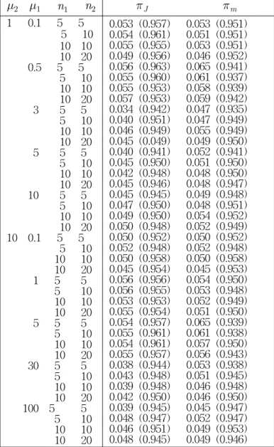
0.05 (0.95) is shown in Table 1.In particular, for fixed
(µ
1, µ
2)
, we take 5,000 independent random samples of X and Y from the model (2). For the cases presented in Table 1, we see that the first order matching prior meets very well the target coverage probabilities for small and moderate values ofn
1 and n2. Note that the Jeffreys' prior does not satisfy the first order matching criterion but its coverage probabilities are compatible to the first order matching prior.Example. The following data, given by Proschan (1963), are time intervals of successive failures of the air conditioning equipment in Boeing 720 aircraft. For aircraft 1, the Bayes estimate of
µ
1 under Jeffrey's prior is 69.95. And the Kolmogorov-Smirnov (K-S) statistic is 0.0835 and its p-value is 0.99. For aircraft 2, the Bayes estimate ofµ
2 under Jeffreys' prior is 94.36. Also the K-S statistic is 0.1699 and its p-value is 0.68. So we can assume that the time between successive failures for each plane is exponentially distributed.Aircraft 1 50 44 102 72 22 39 3 15 197 188 79 88 46 5 5 36 22 139 210 97 30 23 13 14
Aircraft 2 102 209 14 57 54 32 67 59 134 152 27 14 230 66 61 34 Under the Jeffreys' prior and the matching prior, the Bayes estimates and the 95% Bayesian credible intervals of the
θ
1 are -21.15 (-82.08, 27.38) and -21.54 (-81.84, 26.34), respectively. Both of Bayes estimates are similar and length of the confidence interval under the matching prior is shorter than that of the Jeffreys' prior.5. conclusion
In the two exponential distributions, we have found the first order matching prior and Jeffreys' prior for the difference of means. It turns out that the second order matching prior does not exist. And this first order matching prior possesses good frequentist properties in that the coverage probabilities of credible intervals
for the difference of means based on this prior match their frequentist counterpart very closely even for small and moderate sample sizes. Also the Jeffreys' prior does not satisfy the first order matching criterion. From our simulation results and example, we recommend to use the first order matching prior for the Bayesian inference of the difference of two exponential means.
Table 1: Frequentist Coverage Probabilities of 0.05 (0.95) Posterior Quantiles for
θ
1µ
2µ
1n
1n
2π
Jπ
m1 0.1 5 5 5 10 10 10 10 20 0.5 5 5 5 10 10 10 10 20 3 5 5 5 10 10 10 10 20 5 5 5 5 10 10 10 10 20 10 5 5 5 10 10 10 10 20 10 0.1 5 5 5 10 10 10 10 20 1 5 5 5 10 10 10 10 20 5 5 5 5 10 10 10 10 20 30 5 5 5 10 10 10 10 20 100 5 5 5 10 10 10 10 20
0.053 (0.957) 0.053 (0.951) 0.054 (0.961) 0.051 (0.951) 0.055 (0.955) 0.053 (0.951) 0.049 (0.956) 0.046 (0.952) 0.056 (0.963) 0.065 (0.941) 0.055 (0.960) 0.061 (0.937) 0.055 (0.953) 0.058 (0.939) 0.057 (0.953) 0.059 (0.942) 0.034 (0.942) 0.047 (0.935) 0.040 (0.951) 0.047 (0.949) 0.046 (0.949) 0.055 (0.949) 0.045 (0.049) 0.049 (0.950) 0.040 (0.941) 0.052 (0.941) 0.045 (0.950) 0.051 (0.950) 0.042 (0.948) 0.048 (0.950) 0.045 (0.946) 0.048 (0.947) 0.045 (0.945) 0.049 (0.948) 0.047 (0.950) 0.048 (0.951) 0.049 (0.950) 0.054 (0.952) 0.050 (0.948) 0.052 (0.949) 0.050 (0.952) 0.050 (0.952) 0.052 (0.948) 0.052 (0.948) 0.050 (0.958) 0.050 (0.958) 0.045 (0.954) 0.045 (0.953) 0.056 (0.956) 0.054 (0.950) 0.056 (0.955) 0.053 (0.948) 0.053 (0.953) 0.052 (0.949) 0.055 (0.954) 0.051 (0.950) 0.054 (0.957) 0.065 (0.939) 0.055 (0.961) 0.061 (0.938) 0.054 (0.961) 0.057 (0.950) 0.055 (0.957) 0.056 (0.943) 0.038 (0.944) 0.053 (0.938) 0.043 (0.948) 0.051 (0.945) 0.039 (0.948) 0.046 (0.948) 0.042 (0.950) 0.046 (0.950) 0.039 (0.945) 0.045 (0.947) 0.048 (0.947) 0.052 (0.947) 0.046 (0.951) 0.049 (0.953) 0.048 (0.945) 0.049 (0.946)
References
1. Barlow, R.E. and Proschan, F. (1975). Statistical Theory of Reliability and Life Testing. Holt, Reinhart and Winston, New York.
2. Berger, J.O. and Bernardo, J.M. (1989). Estimating a Product of Means : Bayesian Analysis with Reference Priors. Journal of the American Statistical Association, 84, 200-207.
3. Berger, J.O. and Bernardo, J.M. (1992a). Reference Priors in a Variance Components Problem. Bayesian Analysis in Statistics and Econometrics, P. Goel and N.S. Iyengar(eds.). New York: Springer Verlag.
4. Berger, J.O. and Bernardo, J.M. (1992b). On the Development of Reference Priors (with discussion). Bayesian Statistics IV, J.M.
Bernardo, et. al., Oxford University Press, Oxford, 35-60.
5. Bernardo, J.M. (1979). Reference Posterior Distributions for Bayesian Inference (with discussion). Journal of Royal Statistical Society, B, 41, 6. Cox, D.R. and Reid, N. (1987). Orthogonal Parameters and Approximate
Conditional Inference (with discussion). Journal of Royal Statistical Society, B, 49, 1-39.
7. Datta, G.S. and Ghosh, J.K. (1995a). On Priors Providing Frequentist Validity for Bayesian Inference. Biometrika, 82, 37-45.
8. Datta, G.S. and Ghosh, M. (1995b). Some Remarks on Noninformative Priors. Journal of the American Statistical Association, 90, 1357-1363.
9. Datta, G.S. and Ghosh, M. (1996). On the Invariance of Noninformative Priors. The Annal of Statistics, 24, 141-159.
10. Davis, D.J. (1952). An Analysis of Some Failure Data. Journal of the American Statistical Association, 47, 113-150.
11. DiCiccio, T.J. and Stern, S.E. (1994). Frequentist and Bayesian Bartlett Correction of Test Statistics based on Adjusted Profile Likelihood.
Journal of Royal Statistical Society, B, 56, 397-408.
12. Epstein, B. and Sobel, M. (1953). Life Testing. Journal of the American Statistical Association, 48, 486-502.
13. Lawless, J.F. (2003). Statistical Models and Methods for Lifetime Data.
John Wiley and Sons, Inc., Hoboken, New Jersey.
14. Masafumi Akahira (2002). Confidence Intervals for the Difference of Means: Application to the Behrens-Fisher Type Problem. Statistical Papers, 43, 273-284.
15. Mukerjee, R. and Dey, D.K. (1993). Frequentist validity of Posterior Quantiles in the Presence of a Nuisance Parameter : Higher Order Asymptotics. Biometrika, 80, 499-505.
16. Mukerjee, R. and Ghosh, M. (1997). Second Order Probability Matching Priors. Biometrika, 84, 970-975.
17. Proschan, F. (1963). Theoretical Explanation of Observed Decreasing Failure Rate. Technometrics, 5, 375-383.
18. Sang Gil Kang (2004). Noninformative Priors for the Common Scale Parametrer in the Inverse Gaussian Distributions, Journal of the Korean Data & Information Science Society, 15, 4, 981-992.
19. Stein, C. (1985). On the Coverage Probability of Confidence Sets based on a Prior Distribution. Sequential Methods in Statistics, Banach Center Publications, 16, 485-514.
20. Tibshirani, R. (1989). Noninformative Priors for One Parameter of Many. Biometrika, 76, 604-608.
21. Welch, B.L. and Peers, H.W. (1963). On Formulae for Confidence Points based on Integrals of Weighted Likelihood. Journal of Royal Statistical Society, B, 25, 318-329.
[ received date : Sep. 2005, accepted date : Oct. 2005 ]