Predictions of non-uniform tip clearance effects on the flow field in an axial compressor

(1)

Predictions of non-uniform tip clearance effects on the flow field in an axial compressor

Young-Seok Kang

Korea Aerospace Research Institute

115 Gwahangno 45 Eoeun-dong Yuseong-gu Daejon [email protected]

Shin-Hyoung Kang Seoul National University San56-1 Sinlim-dong Gwanak-gu Seoul

[email protected]

Keywords: Compressor, Eccentricity, Alford’s Force

Abstract

Asymmetric tip clearance in an axial compressor induces pressure and velocity redistributions along the circumferential direction in an axial compressor. This paper presents the mechanism of the flow redistribution due to the asymmetric tip clearance with a simple numerical modeling. The flow field of a rotor of an axial compressor is predicted when an asymmetric tip clearance occurs along the circumferential direction. The modeling results are supported by CFD results not only to validate the present modeling but also to investigate more detailed flow fields. Asymmetric tip clearance makes local flow area and resultant axial velocity vary along the circumferential direction. This flow redistribution

‘seed’ results in a different flow patterns according to the flow coefficient. Flow field redistribution patterns are largely dependent on the local tip clearance performance at low flow coefficients. However, the contribution of the main flow region becomes dominant while the tip clearance effect becomes weak as the flow coefficient increases. The flow field redistribution pattern becomes noticeably strong if a blockage effect is involved when the flow coefficient increases. The relative flow angle at the small clearance region decreases which result in a negative incidence angle at the high flow coefficient. It causes a recirculation region at the blade pressure surface which results in the flow blockage. It promotes the strength of the flow field redistribution at the rotor outlet. These flow pattern changes have an effect on the blade loading perturbations. The integration of blade loading perturbation from control volume analysis of the circumferential momentum leads to well-known Alford’s force. Alford’s force is always negative when the flow blockage effects are excluded.

However when the flow blockage effect is incorporated into the modeling, main flow effects on the flow redistribution is also reflected on the Alford’s force at the high flow coefficient. Alford’s force steeply increases as the flow coefficient increases, because of the tip leakage suppression and strong flow redistribution. The predicted results are well agreed to CFD results by Kang and Kang (2006).

Introduction

Non-uniform tip clearance distribution due to compressor shaft offset from its casing center can induce aerodynamic destabilizing rotor dynamic force.

Fig. 1 schematically shows a statically an offset rotor row of a turbomachine. Thomas (1958) and Alford (1965) first announced this finding for axial flow turbines with statically offset rotors to elucidate the tangential destabilizing reaction force, so called Alford or Thomas force. They said Alford’s force is always in the rotational direction of turbine stages. It causes whirl motion of the turbine rotor rows in the direction of rotation (so-called forward whirl). But there was a disparity of the direction of Alford’s force for axial flow compressors. Alford suggested that work is transferred more efficiently from the blade to the fluid in the small clearance region and less efficiently in the large clearance. As a result, Alford’s force has the same direction as rotation and can drive forward whirl of the rotor row. On the contrary, Ehrich (1993) assumed that the blade sustains high pressure difference at the small clearance region and low pressure difference at the large clearance region.

Thus Alford’s force has opposite direction of the rotation (so called backward whirl) based on Ehrich’s theory.

To resolve this disparity in Alford’s force direction, there are several models developed to predict asymmetric tip clearance effects on Alford’s force of axial compressors. Colding et al. (1992) predicted Alford's force using an actuator disc model. They assumed tip clearance penalty on the stage efficiency and implemented it on governing equations of their modeling. They predicted Alford's force is positive at most operating conditions except at low flow coefficients. Ehrich et al. (1993) suggested parallel compressor model to predict Alford's force. He assumed that Alford's force is induced by local tip clearance performance. He used measured pressure rise and blade torque for two tip clearance heights.

The parallel compressor model divides a blade row into two parts; half for the small clearance region and half for the large clearance region. He assumed that half of the compressor follows the compressor performance curve of the compressor with small

(2)

clearance and the other half follows the performance curve of the compressor with large clearance. Then pressure perturbation along the circumferential direction was evaluated and Alford's force was obtained. Song et al. (2000) developed 2CAD model originated from the actuator disc model. The advantage of 2CAD model is that it does not require any experimental data. Flow redistribution around the stage is calculated by predicting tip clearance effects on under-turning of tip leakage flow incorporating with the main flow. Spazkovsky (2000) presented 2SPC model by further investigating flow field perturbation with a control volume analysis.

The models were applied to the low speed research compressor of GE. Their results showed different results to the prediction of Colding et al (1992) which results positive Alford’s force at most flow coefficients. The axial compressor experiences negative Alford's force at most flow coefficients.

Spazkovsky (2000) reported that Alford's force is affected not only by the flow coefficient and but by the blade shape. The blade loading factor shown in Eq.

(1) is defined by perturbing the tangential force acting on the blade surface.

(^tan ^tan ) ¹

2 ₁+ ₂ −

=

Λ^b α β φ (1) It indicates Alford's force direction; negative sign means negative Alford's force and positive sign means positive Alford's force. Since the rotor inlet flow angle and rotor outlet blade angle are nearly constant, Alford's force reverses as the flow coefficient according to the blade loading factor.

Previous researches have shown that flow redistribution and Alford’s force variation are largely dependent on the flow coefficient. However, it is not fully understood the mechanism of the flow redistribution and Alford's force variation according to the flow coefficient. Therefore, in this paper, we developed a simple modeling which predicts flow

field redistributions along the circumferential direction of the rotor row. Also the present study aims to find a source of the flow redistribution and mechanism of Alford's force reversal according to the flow conditions.

Model Derivation

The flow field at the inlet and outlet of the rotor row is predicted by integrating governing equations along the streamline as shown in Fig. 2. The modeling requires following assumptions to simplify complicated 3-D flow to 2-D flow at the inlet and outlet of an axial compressor.

1. Tip clearance distribution is a sinusoidal function when the rotating axis is offset from the casing center.

2. Assuming that there are three major total pressure loss sources; Incidence loss due to incidence angle, tip clearance loss from tip leakage flow and its mixing with the main flow and profile loss due to flow dissipation. Incidence pressure loss due to large incidence or negative incidence has an important role in this modeling. Tip clearance loss is varied along the circumferential direction due to non-uniform tip clearance distributions. In this modeling, total pressure loss including these three losses is treated as a source term.

3. Deviation angle and under-turned angle due to tip leakage flow of the axial compressor are evaluated from Howell’s compressor cascade theory.

e₀ F_Y

ω

x y

e₀ F_Y

ω

x y

Fig. 1 Schematic diagram of a statically offset rotor row of turbomachine

α1

β1

U

α2

β2

U 2 : Blade Outlet

βb

1 : Blade Inlet

h s

s h hδ

∂ +∂

W1 W2

W1

W2

α1

β1

U α1

β1

U

α2

β2

U α2

β2

U 2 : Blade Outlet

βb

1 : Blade Inlet

h s

s h hδ

∂ +∂

W1 W2

W1

W2

Fig.2 Control surface of the rotor row for the model

(3)

4. There can be an effective flow area change due to asymmetric tip clearance or blockage. This can be treated as an equivalent eccentricity from the casing center.

Continuity Equation

As there is an asymmetric tip clearance distribution along the circumferential direction, the continuity equation is written as follows

1 0

∂ = +∂

∂

∂ s W t h

h (2)

( ₀ )sinθ

0 e eb

h

h= − + (3)

Where, h is blade height, e₀ is a statically offset distance and eb is an equivalent offset distance due to blockage effect which will be explained later. It means the relative velocity along the streamline accelerates or decelerates according to the local blade height. It is convenient to convert the continuity equation into a velocity dimension. Tip equivalent velocity q is defined as

h

q=ω (4)

The continuity equation can be rewritten as follows.

=0

∂ + ∂

∂

s q W t

q (5)

Momentum Equation

The meridional momentum equation includes a source term, which is total pressure loss between the inlet and outlet of the rotor row.

s s p s

W W t

W −

∂

− ∂

∂ = + ∂

∂

ρ

1 (6)

Adding Eq. (5) to Eq. (6) and integrate the equation from the inlet to the outlet to solve the equation.

ds s s p

s ds q W s W W t q t W

∫

⎟⎟⎠

⎜⎜ ⎞

⎝

⎛ +

∂

− ∂

=

⎟⎠

⎜ ⎞

⎝

⎛

∂ + ∂

∂ +∂

∂

2 1 2 1

1 ρ

(7)

The first term of the integrated equation is modified in forms of

e m m

b

m b

C L t

C

A ds A t ds C

t W

⎟⎟⎠

⎜⎜ ⎞

⎝

⎛

∂ + ∂

∂ ′

= ∂

∂

= ∂

∂

∫

ω θ β

β

2 2

2

1 2

2 2 1

cos 1

(8)

Whereβ is the mean blade angle, _b L_eis an equivalent stream line length from the inlet and outlet. As investigating a flow field in the global coordinate is convenient in this study, conversion into the global coordinates is required for the time derivates terms of Eq. (7)

ω θ θ

θ

∂ + ∂

′

∂

=∂

∂

′

∂ +∂

′

∂

=∂ ² ² ² ²

2 m m m m

m C

t C C

t t C dt

dC (9)

At the rest part of this paper, the dot at the right hand side of Eq. (9) will be omitted for convenience. In a similar manner forth term of in Eq. (7) becomes,

( )^ω ^θ

ω θq e₀ e_b ²cos t

q =− +

∂

= ∂

∂

∂ (10)

As q is the function of θ , there is no necessity of a time derivate in the global coordinate. From the Euler-Turbine Equation, the third term of Eq. (7) becomes

( )

(

1²

)

2 2 1 2 2

1 2

1 C C

C C U s ds

W W =− _t − _t + −

∂

∫

∂ (11)

With the mean blade angle, last part of the left-hand side of Eq. (7) becomes,

b d m

b

q C s ds q C

sds q W

β

β cos

cos

1 ²

1 2

1 ≈

∂

= ∂

∂

∂ ∫

∫ (12)

Cd in Eq. (12) is the axial velocity difference between control volume inlet and outlet. Then final equation becomes,

( ) ( )

θ β ω

ρ β

ω θ

cos cos ) (

1 cos

2 0

01 02 1 2 2 2

b b

l d t

t e

b m m

e e

S qC p p C C L U

C t C

+ +

⎭⎬

⎫

⎩⎨

⎧ − − − − −

=

∂ + ∂

∂

(13)

Blockage Effect

Kang (2006) showed that large back flow region appears at the pressure side of the rotor blade as the flow coefficient increases. In this study, the flow blockage is assumed to be imposed on the casing

( )

(

o b i

) (

o i

)

o b

b r e r r r re

A

A−δ =π − ²− ² =π ²− ² −2π (14)

( )

⎟⎟

⎠

⎞

⎜⎜

⎝

⎛

⎟⎟⎠

⎞

⎜⎜⎝

−⎛

− =

= 2 2 2

1 2 2

o i o b

i o

b o b

r r r e

r r

e r A

A π

π

δ (15)

Where δA_b is a flow area decrease due to the blockage and e means the equivalent offset. To _b quantify a flow blockage is to predict the maximum

(4)

difference of the axial velocity at the rotor outlet.

Kang showed that the axial velocity variations, difference between maximum and minimum axial velocity normalized by blade rotational speed. One can easily assume that the velocity variation is inversely proportional to the flow blockage. A linear increase appears when the flow coefficient is over 0.425. Therefore the equivalent eccentricity due to the blockage can be linearized as a function of the flow coefficient as Eq. (16).

B A

e_b= φ+ (16) To determine e in Eq. (15), Roelke’s correlation in _b Eq. (17) is used. Refer to Roelke (1994) for details.

i i

i A

A_b

cos sin

sin

= +

δ (17)

Deviation Angle and Under-Turned Flow due to Tip clearance

Fluid flow leaving the rotor blade deviates from the exit blade angle due to pressure difference between pressure and suction surfaces. Another source that affects flow angle is tip clearance flow which results in under-turned flow relative to the main flow. As the tip clearance height and flow area varies along the circumferential direction, blade loading and tip clearance flow also changes corresponding to the local location. In this modeling, it is assumed that blade loading and corresponding deviation angle follow Howell’s cascade theory (Howell, 1942, 1945).

(² ^/ ) ^/⁵⁰⁰

23 .

0 × ²+β₂^*

= a l

m (18)

( )s/ l ²¹ θm

δ = (19)

From the above two equations, the deviation angle at the nominal flow condition is evaluated. Deviation angles at the rest flow coefficients are evaluated based on the Howell’s empirical formulations. The lift coefficient can be evaluated using Eq. (20).

( ) d b

b

l c

l

c =2scosβ tanβ₁−tanβ₂ − tanβ (20)

where c_d is an empirical formulation of the drag coefficient of the compressor cascade suggested by Howell (1942).

Since the tip clearance flow at the axial compressor is usually assumed to be inviscid flow, the speed of tip clearance flow can be evaluated from the pressure difference between the pressure and suction surfaces.

ρ

ss ps gap

p

W p −

= 2 (21)

The under-turned flow angle can be predicted as

l gap

t c

W

W ₁

1 tan

tan⁻ = ⁻

θ = (22)

Loss Model

In this study, the model employs tip leakage, incidence and resultant secondary flow and profile losses in Eq. (23) for reasonable predictions of the flow fields in the rotor row.

( t i p)

l U L L L

S = ² + +

21 ρ (23)

Tip clearance loss is modeled by modifying Storer’s modeling (1993) for compressor cascades.

2 2 2

2

cos 1 )

sin 1 (

cos 2 sin sin 2

β θ

χ

θ θ

θ χ χ

φ ⎪⎭

⎪⎬

⎫

⎪⎩

⎪⎨

⎧ +

−

= +

t t t

t

Lt (24)

Where χ is tip clearance area to flow area ratio.

Incidence loss follows Roelke’s suggestion (1994) that the kinetic energy normal to blade passage becomes loss.

U i Li W

2 2

⎟ sin

⎠

⎜ ⎞

⎝

=⎛ (25)

Profile loss is assumed to be proportional to the kinetic energy in the flow passage.

2

⎟⎠

⎜ ⎞

⎝

= ⎛ U K W

Lp p (26)

Solving Equation

Eq. (13) is a first-order hyperbolic equation to solve forCm₂,

C S t

C_m _m =

∂ + ∂

∂

ω θ²

2 (27)

To discretize Eq. (13), Lax-wendroff scheme is used, which is 1^st order in time and 2^nd order in space.

Discrete form of Eq. (13) is obtained as

( )

(

^C ^C ^C

)

^S

CFL

C CFL C

C C

k i m k

i m k

i m

k i m k

i m k

i m

+ − + +

−

=

− +

− + +

1 , 2 , 2 1 , 2 2

1 , 2 1 , 2 ,

2 1 , 2

2 2

2 (28)

where CFL=ωΔt/Δθ. Axial velocity at the inlet is from,

1 , 2 1 , 1

+ + = _m^k _i

k i

m C

C (29)

The inlet circumferential velocity is evaluated from the velocity triangle. It is assumed that the tip

(5)

clearance region and main flow region contributions are separated according to the tip clearance height.

1 1 , 1 1 ,

1⁺ = _m^k⁺_itanα

k i

t C

C (30)

( ) ( )_⎟⎟

⎠

⎜⎜ ⎞

⎝

⎛ − +

+ +

−

= ⁺

+

i b i i

t b i k

i m k

i

t h

h h h

C h U

C sin β θ sin β δ

0 0 , 0

1 , 1 1

, 2

(31)

Subtracting dynamic pressure from total pressure becomes static pressure at the inlet and outlet.

(

2 ²1,

)

, 1 01

,

1 2

1

i t i m i

s p C C

p = − ρ + (32)

( t i t i)

(

m i t i

)

l

i

s U C C C C s

p₂_, = ₂_, − ₁_, − ²₁_, + ²₁_, − 21 ρ

ρ (33)

0 0.2 0.4 0.6 0.8 1

0.38 0.40 0.42 0.44 0.46 0.48 0.50 0.52

-0.02 -0.01 0.00 0.01 0.02

0 0.2 0.4 0.6 0.8 1

0.38 0.40 0.42 0.44 0.46 0.48 0.50 0.52

-0.02 -0.01 0.00 0.01 0.02

0 0.2 0.4 0.6 0.8 1

0.16 0.18 0.20 0.22 0.24 0.26

-0.02 -0.01 0.00 0.01 0.02

0 0.2 0.4 0.6 0.8 1

-0.56

-0.54

-0.52

-0.50

-0.48

-0.46

-0.44

-0.42 -0.02

-0.01 0.00 0.01 0.02

0 0.2 0.4 0.6 0.8 1

-0.10 -0.05 0.00 0.05 0.10

-0.02 -0.01 0.00 0.01 0.02

0 0.2 0.4 0.6 0.8 1

-0.10 -0.05 0.00 0.05 0.10

-0.02 -0.01 0.00 0.01 0.02

Normalized Axial Velocity Normalized Axial Velocity

Normalized Circumferential Velocity Normalized Circumferential Velocity

Normalized Pressure Perturbation Normalized Pressure Perturbation

(a)

(b)

Normalized Circumferential Location (c) Normalized Circumferential Location Normalized Circumferential Location Normalized Circumferential Location Normalized Circumferential Location Normalized Circumferential Location

At the blade inlet At the blade outlet

CFD results at Φ=0.400 CFD results at Φ=0.480 Predicted result at Φ=0.400 Predicted result at Φ=0.480 Tip Clearance Distributions

CFD results at Φ=0.400 CFD results at Φ=0.480 Predicted result at Φ=0.400 Predicted result at Φ=0.480 Tip Clearance Distributions CFD results at Φ=0.400

CFD results at Φ=0.480 Predicted result at Φ=0.400 Predicted result at Φ=0.480 Tip Clearance Distributions

CFD results at Φ=0.400 CFD results at Φ=0.480 Predicted result at Φ=0.400 Predicted result at Φ=0.480 Tip Clearance Distributions CFD results at Φ=0.400

CFD results at Φ=0.480 Predicted result at Φ=0.400 Predicted result at Φ=0.480 Tip Clearance Distributions

CFD results at Φ=0.400 CFD results at Φ=0.480 Predicted result at Φ=0.400 Predicted result at Φ=0.480 Tip Clearance Distributions

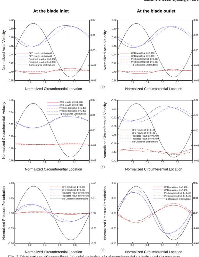
Fig. 3 Distributions of normalized (a) axial velocity, (b) circumferential velocity and (c) pressure perturbations at the inlet and outlet

(6)

Modeling Results

The model is implemented in an analysis for the 3^rd stage rotor row of a low speed research compressor (LSRC) in Seoul National University. It is 2/3 scaled down model from LSRC operated in GE (Wisler et al. 1981). Table 1 gives brief specification of the LSRC. The modeling results are compared to computationally calculated results by Kang and Kang (2006). They carried out numerical simulations for the rotor row with a static offset from the casing center.

The inlet and outlet flow redistribution results are available to compare with modeling results. Refer to Kang and Kang (2006) for details of numerical simulation process.

Velocity and pressure distributions

Fig. 3 shows velocity and pressure distributions at the inlet and outlet for the flow coefficient of 0.400 and 0.480. The flow coefficient of 0.400 is near the design flow coefficient. It is known that Alford’s force has a positive value at the high flow coefficient (Storce, 2000 and Ehrich, 2000). Therefore, the result at 20% higher flow coefficient than the design flow coefficient is compared. The predicted results are compared to the numerical simulation results by Kang (2006). The axial velocity is high at the small clearance region and small at the large clearance region at both flow coefficients. The blockage effect promotes amplitude of axial velocity variation when the flow coefficient is 0.480 and it also affects circumferential velocity and static pressure. For both predicted and calculated results, there is little phase difference between tip clearance distribution and flow redistributions when the flow coefficient is 0.400. But small discrepancy appears when the flow coefficient is 0.480. The predicted circumferential velocity at the blade inlet and outlet shows a good agreement with the calculated results. It means it is proper assumptions that the rotor blade follows Howell’s cascade theories which determine the outlet flow angle at the nominal and off-design conditions.

Pressure variations are shown in Fig. 3 (c) for both flow coefficients. However, the reason of pressure variation is different for each case. As shown in Fig. 3 (a), a large axial velocity variation occurs at high flow coefficients while relatively small amount of velocity variation occurs at low flow coefficients.

Kang reasoned that the tip leakage flow is dominant over the local pressure rise when the flow coefficient is small. The pressure loss at the large clearance

region is higher than that of the small clearance.

Therefore, small clearance region has its maximum value and large clearance has its minimum value. As the flow coefficient increases, the tip leakage has little effect on the flow. The flow blockage due to the local velocity triangle variation and corresponding local pressure rise becomes the major effect on the pressure redistribution along the circumferential direction.

Therefore pressure distribution pattern reverses compared to that of the design or small flow coefficients. Next section details the flow mechanism changes according to the flow coefficient.

Alford’s force distributions

Fig. 4 compares Alford’s force distributions from the numerical simulation and predicted results.

Alford’s force is evaluated by integrating circumferential force perturbation which is from the circumferential momentum conservation equation. In Fig. 4, both numerical simulation and predicted Alford’s force are negative when the flow coefficient is 0.400. Both Alford’s forces change their signs where the flow coefficient is approximately 0.445.

Alford’s force prediction without the flow blockage is compared. Predicted Alford’s force shows negative value at the all flow coefficient if the flow blockage is not considered.

If there is no area difference between the small clearance region and large clearance region, there would be no axial velocity difference. However, there is an axial velocity variation as shown in Fig. 5 (a) between the small clearance and the large clearance due to a flow area difference. If the axial velocity variation does not change according to the flow coefficient, pressure rises at the small and large clearance vary as shown in Fig. 5 (a). In this case, the rotor row experiences high blade loading at the small clearance region and low blade loading at the large clearance region expect for very high flow coefficients.

The pressure difference becomes small as the flow coefficient increases. When the flow coefficient reaches a certain point, there is no difference in the pressure difference between the small clearance and large clearance disappears. At the point, there is no pressure perturbation around the rotor row and resultant Alford’s force becomes zero. When the flow coefficient is higher than this ‘thresholds flow coefficient”, little difference occurs in the pressure rise occurs between the small clearance and large clearance. In opposition to the low flow coefficients, the pressure rise pattern reverses; low pressure rise at the small clearance and high pressure rise at the large clearance. Therefore the sign of Alford’s force reverses at the higher flow coefficient than the

‘thresholds flow coefficient’.

However, if the blockage concept in the present study is introduced in the model, the axial velocity difference becomes large as the flow coefficient increases as shown in Fig. 5 (b). Therefore the threshold flow coefficient becomes a smaller value than that of Fig. 5 (a). Large axial velocity difference Table 1 Brief specification of the rotor blade

Radius (cm) 70.45

Chord (cm) 9.55

Solidity 1.163 Stagger angle (deg) 33.09

tmax/c 0.062

No. of Blades 54

(7)

and small threshold flow coefficient induce higher pressure difference or blade loading as shown in Fig.

5 (b). Resultant Alford’s force increases rapidly at the high flow coefficient region. It well explains why the main flow region is more influential than tip clearance region in redistributing velocity and pressure field around the rotor row in both numerical simulation and predicted results.

The results show that conventional axial compressors may have negative value of Alford’s force at the most operating conditions. But other factors such as a flow blockage due to large flow incidence or secondary flow, tip leakage flow would be dominant factors at the high flow coefficient. It is possible in case of an axial type of fan. It has a low solidity and may suffer more secondary flow. In this case, the axial flow turbo-machine would have positive Alford’s force even at the operating point.

Conclusion

1. A numerical modeling was developed to predict an asymmetric tip clearance effect on an axial compressor rotor row. The predicted results are well agreed with numerical simulation results. Not only the statically offset distance, but also other factors such as a tip leakage flow or a flow blockage have important roles on the reasonable prediction of the asymmetric tip clearance effects. It means it is hard to assess the asymmetric tip clearance effects with geometry information alone when these factors have noticeable contributions.

2. When the flow coefficient is low, velocity and pressure redistributions are largely dependent on the local tip clearance performance. As the tip clearance effect according to tip clearance heights becomes very small at the high flow coefficient, the determinant factor which redistribute flow field around the rotor row is local main flow performance according to the local axial velocity.

3. Like previous researches, Alford’s force in the rotor was negative value at low flow coefficients.

However with the blockage and tip leakage flow, Alford’s force, the threshold flow coefficient moves to low flow coefficient region. The blockage effect

promotes a steep increase in Alford’s force at the high flow coefficient.

Nomenclature C : Absolute velocity [m/s]

cP : Pressure coefficient

e0 : Eccentricity of asymmetric tip clearance [m]

eb : Equivalent eccentricity of flow blockage [m]

i : Incidence angle [deg]

h : Blade height [m]

l : Blade chord length [m]

L : Loss coefficient

FT : Tangential force acting on blades [N]

q : Tip equivalent velocity [m/s]

p : Pressure [pa]

R : Radius [m]

s : Stream-wise direction, Source term U : Rotor tip velocity [m/s]

W : Relative velocity [m/s]

α : Absolute flow angle [rad]

Negative Alford’s force Positive Alford’s force

Alford’s Force (N)

Flow Coefficient

Prediction with blockage Prediction without blockage CFD results

0.38 0.4 0.42 0.44 0.46 0.48 0.5

-10 -5 0 5 10 15 20

Fig. 4 Alford’s force distributions

Negative Alford’s force

Positive Alford’s force

Threshold flow coefficient

(b) (a)

U C Cm,max− m,min

Small clearance

Nominal clearance

Large clearance

Pressure Rise Coefficient

(b) (a)

U C Cm,max− m,min

Small clearance

Nominal clearance

Large clearance

Fig. 5 Schematics of asymmetric tip clearance effects on pressure rise (a) without and (b) with a flow blockage

(8)

β : Relative flow angle [rad]

β : Mean blade angle [rad] b

φ : Flow coefficient ρ : Density [kg/m³]

θ : Circumferential coordinate ω : Rotational speed [rad/s]

Subscript

0 : Nominal value, total condition 1 : Rotor inlet

2 : Rotor outlet m : Axial direction s : Static condition

t : Circumferential direction References

1) Alford, J., 1965, "Protecting Turbomachinery from Self-Excited Rotor Whirl, Journal of Engineering for Power, pp. 333-344.

2) Thomas, H. J., 1958, "Unstable Natural Vibration of Turbine Rotors Induced by the Clearance Flow in Glands and Blading", Bull. de l'A.I.M., Vol. 71, No.11/12, pp. 1039-1063

3) Vance, J. M. and Laudadio, F. J., 1984,

"Experimental Measurement of Alford's Force in Axial Flow Turbomachinery", ASME Journal of Engineering for Gas Turbines and Power, Vol.

106, pp.585-590

4) Colding-Jorgensen, J., 1992, "Prediction of Rotordynamic Destabilizing Forces in Axial Flow Compressors", Journal of Fluid Engineering, Vol.

114, pp.621-625

5) Ehrich, F.F., 1993, “Rotor Whirl Forces Induced by the Tip Clearance Effect in Axial Flow Compressors”, Journal of Vibration and Acoustics, Vol. 115, pp. 509-515

6) Ehrich, F.F et al, “Unsteady Flow and Whirl- Inducing Forces in Axial-Flow Compressors. Part II – Analysis”, ASME/IGTI TurboExpo 2000, Munich, Germany.

7) Howell, A. R. 1942, “The Present Basis of Axial Flow Compressor Design: Part I, Cascade Theory and Performance”, ARC R and M. 2095

8) Howell, A. R. 1945, “Design of Axial Compressor”, Proc. Inst. Mech. Engrs., 153.

9) Howell, A. R. 1945, “Fluid Dynamics of Axial Compressors”, Proc. Inst. Mech. Engrs., 153.

10) Kang, Y.S., and Kang, S.H., 2005, “Prediction of the Fluid induced instability Force of an axial compressor”, ASME FEDSM 2006, Miami, FL.

11) Roelke, R. J., “"Miscellaneous Losses,”" Chapter 8 of Turbine Design and Applications, NASA SP- 290, Glassman, A. J., ed., 1994.

12) Song, S.J., and Cho, S.H., 2000, “Non-uniform Flow in a Compressor due to Asymmetric Tip Clearance”, ASME/IGTI TurboExpo 2000, Munich, Germany.

13) Spakovszky, Z. S., 2000, “Analysis of Aerodynamically InducedWhirling Forces in Axial

Flow Compressors”, ASME/IGTI TurboExpo 2000, Munich, Germany.

14) Storace, A.F et al, 2000, “Unsteady Flow and Whirl-Inducing Forces in Axial-Flow Compressors. Part I – Experiment”, ASME/IGTI TurboExpo 2000, Munich, Germany.

15) Storer, J. A. and Cumsty, N. A., "An approximate Analysis and Prediction Method fot Tip Clearance Loss in Axial Compressors", ASME Paper, 93- GT-140

16) Wisler, D. C., 1981, “Compressor Exit Stage Study Volume IV - Data and Performance Report for the Best Stage,” NASA CR-165357.