Spatial Distribution Pattern of Chloranthus japonicus Population at Mt. Ahop
Man Kyu Huh*
Division of Applied Bioengineering, Dong–eui University, Busan 47340, Korea
Received September 22, 2017 /Revised October 13, 2017 /Accepted October 20, 2017
The patchiness of local environments within a habitat is assumed to be a primary factor affecting the spatial patterns of plants, and a randomization procedure is developed for testing the null hypothesis that only spatial association with patches determined the spatial patterns of plants. Chloranthus japoni- cus (Chloranthaceae) is an herbaceous perennial and a member of the genus Chloranthus in the family Chloranthaceae. The spatial pattern of C. japonicus was analyzed according to several patchiness in- dices, population uniformity or aggregation under different sizes of plots by dispersion indices, and spatial autocorrelation. Population densities (D) varied from 0.356 to 2.270, with a mean of 1.527. The values of dispersion indices ( at Mt. Ahop were lower than 1 at six plots (2 m × 2 m, 2 m × 4 m, 4 m × 4 m, 4 m × 8 m, 8 m × 8 m, and 8 m × 16 m), but the two large plots (16 m × 16 m and 16 m
× 32 m) were higher than 1. Thus, the aggregation indices ( were negative at Mt. Ahop, which in- dicates a uniform distribution. The two large plots (16 m × 16 m and 16 m × 32 m) had positive CIs.
However, the values were not large (0.009 for the 16 m × 16 m plot and 0.038 for the 16 m × 32 m plot). The mean crowding (M*) and patchiness index (PAI) showed positive values for all plots.
Key words : Chloranthus japonicus, Mt. Ahop, mean crowding, patchiness index, spatial distribution
*Corresponding author
*Tel : +82-51-890-1529, Fax : +82-505-182-6870
*E-mail : [email protected]
This is an Open-Access article distributed under the terms of the Creative Commons Attribution Non-Commercial License (http://creativecommons.org/licenses/by-nc/3.0) which permits unrestricted non-commercial use, distribution, and reproduction in any medium, provided the original work is properly cited.
Journal of Life Science 2018 Vol. 28. No. 2. 148~152 DOI : https://doi.org/10.5352/JLS.2018.28.2.148
Introduction
Spatial distribution pattern of suitable environments for plants is often patchily structured at various sizes within the habitat, like islands in a sea [10]. The word "structure"
comes from Latin struere which means to build, to arrange, and contains the notion of an organized thing. Performances of individual plants in response to the patchiness of environ- ments are spatially non-random processes [19], such as den- sity-independent mortality [2], patchy establishment of seed- lings [4] and seed dispersal patterns within and between patches [18].
Spatial structures exist, because geographical space is not constituted by a set of unique places, occupying random locations. A spatial structure is completely described only if, beyond the form taken by the arrangement of objects, it is possible to figure out the inter-dependencies among the latter. Spatial structuring is an essential community and eco- system property [20]. Understanding the underlying causes
of community composition and its spatial variation (E-diver- sity) remains a major goal in community ecology [8, 12].
Species distribution is not to be confused with dispersal, which is the movement of individuals away from their area of origin or from centers of high on density. Dispersion or distribution patterns show the spatial relationship between members of a population within a habitat. Individuals of a population can be distributed in one of three basic pat- terns: uniform, random, or clumped. In a uniform dis- tribution, individuals are equally spaced apart, as seen in negative allelopathy where chemicals kill off plants sur- rounding sages. In a random distribution, individuals are spaced at unpredictable distances from each other, as seen among plants that have wind-dispersed seeds. In a clumped distribution, individuals are grouped together, as seen among elephants at a watering hole.
Chloranthus japonicus Siebold is a perennial plants and ge- nus is Chloranthus in the family Chloranthaceae. The Chlo- ranthaceae is a small family with five genera and around seventy species occurring in tropical America, East Asia and the Pacific [13]. C. japonicus is an unusual and rare shade perennial that emerges in early spring with warm burgundy stems with a whorl of four mid green, textured, slightly shi- ny, serrated leaves each about 3-5 inches long topped with a short spike of feathery white flowers [14]. Flowers are white and flowering in March to April.
The purpose of this paper was to describe a statistical analysis for detecting a species association, which is valid even when the assumption of within- species spatial ran- domness is violated. The present study used the point pat- tern analysis method to investigate the variation in the spa- tial distribution pattern of C. japonicus at different spatial scales and spatial autocorrelation at different plots in a 16
× 32 m2 spatial scales at the Mountain Ahop in Korea.
Materials and Methods
Surveyed regionsThis study was carried out on the populations of C. japoni- cus, located at Mt. Ahop (346.5 m) (35°16‘N/129°11’E) in Busan-ci (Korea). The elevation of community of C. japonicus ranges from 210 to 245 m. The site is characterized by a temperate climate with a little hot and long summer. In this region the mean annual temperature is 14.7℃ with the max- imum temperature being 29.4℃ in August and the minimum -0.6℃ in January. Mean annual precipitation is about 1519.1 mm with most rain falling period between June and August.
Sampling procedure
Many quadrats at Mt. Ahop were randomly chosen for each combination of site x habitat, so that, overall, 50 quad- rats were sampled for the complete experiment. Spatial ecol- ogists use artificial sampling units (so-called quadrats) to de- termine abundance or density of species. The number of events per unit area are counted and divided by area of each square to get a measure of the intensity of each quadrat.
I randomly located quadrates in each plot which I estab- lished populations. The quadrat sizes were 2 m × 2 m, 2 m
× 4 m, 4 m × 4 m, 4 m × 8 m, 8 m × 8 m, 8 m × 16 m, 16 m × 16 m, and 16 m × 32 m.
Index calculation and data analysis
Given the above definition of spatial autocorrelation, it is expected that the x–y coordinates of points (e.g. in- dividual plants) having a spatial structure are more likely to be spatially close than expected by chance alone.
Following this simple idea, the nearest neighbor method measures the mean nearest distance for all points di, where i =1 for the first neighbor [21]. The spatial pattern of C. japo- nicus was analyzed according to the Neatest Neighbor Rule [3, 15].
Average viewing distance (rA) was calculated as follows:
The ri is the distance from the individual to its nearest neighbor individual. N is the total number of individuals within the quadrat.
The expectation value of mean distance of individuals within a quadrat (rB) was calculated as follows:
Where D is population density and the number of in- dividuals per plot size.
R = rA/ rB
The significance index of the deviation of R that departs from the number of “1” is calculated from the following for- mula [15].
One test for spatial pattern and associated index of dis- persion that can be used on random-point-to-nearest-organ- ism distances was suggested by Eberhardt [5] and analyzed further by Hines and Hines [11]: IE= (s/m)2+ 1
Where IE = Eberhardt’s index of dispersion for point-to-or- ganism distances, s = observed standard deviation of dis- tances, m = mean of point-to-organism distances. Many spa- tial dispersal parameters were calculated the degree of pop- ulation aggregation under different sizes of plots by dis- persion indices: index of clumping or the index of dispersion (C), aggregation index (CI), mean crowding (M*), patchiness index (PAI), negative binominal distribution index K, Ca in- dicators (Ca is the name of one index) [16] and Morisita in- dex (IM) were calculated with Microsoft Excel 2014. The for- mulae are as follows:
Index of dispersion: C = S2/ m Aggregation index
Mean crowding Patchiness index Aggregation intensity Ca indicators Ca = 1 / k IM =
Where S2 is variance and m is mean density of plants.
The mean aggregation number to find the reason for the aggregation of C. japonicus was calculated [1].
Where r is the value of chi-square when 2 k is the degree
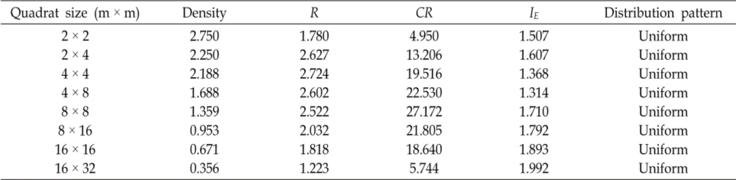
Table 1. Spatial patterns of Chloranthus japonicus individuals at different sampling quadrat sizes in Mt. Ahop
Quadrat size (m× m) Density R CR IE Distribution pattern
2× 2 2× 4 4× 4 4× 8 8× 8 8× 16 16× 16 16× 32
2.750 2.250 2.188 1.688 1.359 0.953 0.671 0.356
1.780 2.627 2.724 2.602 2.522 2.032 1.818 1.223
4.950 13.206 19.516 22.530 27.172 21.805 18.640 5.744
1.507 1.607 1.368 1.314 1.710 1.792 1.893 1.992
Uniform Uniform Uniform Uniform Uniform Uniform Uniform Uniform
Table 2. Changes in gathering strength of Chloranthus japonicus at different sampling quadrat sizes Quadrat size
(m× m)
No.
Quadrat
Aggregation indices
C CI M* PAI PI Ca IM
2× 2 2× 4 4× 4 4× 8 8× 8 8× 16 16× 16 16× 32
16 10 8 6 5 2 2 1
0.433 0.531 0.339 0.331 0.768 0.892 1.009 1.038
-0.566 -0.469 -0.661 -0.669 -0.232 -0.108 0.009 0.038
0.024 0.407 0.259 0.387 0.850 1.018 1.139 1.084
0.040 0.465 0.282 0.366 0.785 0.904 1.008 1.037
-1.042 -1.867 -1.392 -1.579 -4.659 -10.443 122.820 27.369
-0.960 -0.536 -0.718 -0.634 -0.215 -0.096 0.008 0.037
0.047 0.496 0.291 0.371 0.794 0.911 1.014 1.042 of freedom and k is the aggregation intensity. Green index
(GI) is a modification of the index of cluster size that is in- dependent of n [9].
Results and Discussion
Population densities (D) varied from 0.356 to 2.270, with a mean of 1.527(Table 1). Small quadrate sizes such as 2 m
× 2 m, 2 m × 4 m, and 4 m × 4 m have relatively high D values (>2), whereas larger or wider quadrate sizes such as 8 m × 16 m, 16 m × 16 m, and 16 m × 32 m have, com- paratively, very low D values (<1). The values (R) of spatial distance (the rate of observed distance-to-expected distance) among the nearest individuals were higher than 1 and the significant index of CR was >2.58. If by this parameter, the all plots (2 m × 2 m, 2 m × 4 m, 4 m × 4 m, 4 m × 8 m, 8 m × 8 m, 8 m × 16 m, 16 m × 16 m, and 16 m × 32 m) of C. japonicus at Mt. Ahop were uniformly distributed in the forest community. Thus, C. japonicus were not aggregately distributed in this Mt. Ahop population. The expected value of IE in a random population is 1.27. Values below this sug- gest a regular pattern, and larger values indicate clumping.
IE values for all quadrates are larger than 1.27. Under the hypothesis, population of C. japonicus is clumping. Clumped
dispersion is often due to an uneven distribution of nutrients or other resources in the environment. It can also be caused by social interactions between individuals. Additionally, in organisms that don't move, such as plants, offspring might be very close to their parents and show clumped dispersion patterns. Patchy seed dispersal near the mother plants ex- plains the aggregation of seedlings around reproductive plants [6, 7].Within a single habitat, some areas are more ideal to live in than others because they have more food, water, sunlight, or other resources. This can cause many in- dividuals of a population to accumulate in this ideal location.
The values dispersion index (C) at Mt. Ahop were lower at six plots (2 m × 2 m, 2 m × 4 m, 4 m × 4 m, 4 m × 8 m, 8 m × 8 m, and 8 m × 16 m) than 1 except two large plots (16 m × 16 m and 16 m × 32 m) (Table 2). Thus these ag- gregation indices (CI) were negative at Mt. Ahop, which in- dicate a uniform distribution. Two large plots (16 m × 16 m and 16 m × 32 m) were positive. However the values were not large (0.009 for 16 m × 16 m and 0.038 for 16 m × 32 m). The mean crowding (M*) and patchiness index (PAI) showed positive values for all plots. When the three indices C, M*, PAI were <1 and their values of PI and Ca were also shown smaller than zero, it means uniform distributed. In
Fig. 1. The mean aggregation number to find the reason for the aggregation of Chloranthus japonicus.
Fig. 2. The curves of patchiness in two areas of Chloranthus japo- nicus using values of Green index.
C. japonicus, the two indices, C, PAI were >1 and their values of PI and Ca were also shown greater than zero, thus it means aggregately distributed. Thus, two large plots (16 m × 16 m and 16 m × 32 m) of C. japonicus at Mt. Ahop were clustered.
The results were inconsistent with the previous results. One of the reasons is in uneven collection and distribution pat- tern of the C. japonicus was quadrat-sampling dependent.
Morisita index (IM) is related to the patchiness index (PAI) and showed an overly steep slope at the plot 2 m × 4 m.
The values of δ were varied from 0.018 for 16 m × 16 m to 1.284 for 4 m × 8 m (Fig. 1). The values of δ showed a tendency to decrease as the plot size increased. As Morisita’s coefficient estimates spatial distribution pattern using the mean and variance of each sampling date separately, so this index is more perfect than dispersion index [17]. The de- tailed knowledge of dispersion in different time intervals during growing season would be useful for research strat- egies more than management programs. When the area was larger than 16 m × 16 m, the degree of aggregation increased significantly with increasing quadrat sizes, while the patchi- ness indices did not change from the plot 4 m × 4 m to 4 m × 8 m. Green index varied between -0.561 to 0.213 (Fig. 2).
References
1. Arbous, A. G. and Kerrich, J. E. 1951. Accident statistics and the concept of accident proneness. Biometrics 7, 340-342.
2. Casper, B. B. and Cahill, Jr. J. F. 1996. Limited effects of soil nutrient heterogeneity on populations of Abutilon theo- phrasti (Malvaceae). Am. J. Bot. 83, 333-341.
3. Clark, P. J. and Evans, F. C. 1954. Distance to nearest neigh- bor as a measure of spatial relationships in populations.
Ecology 35, 445-453.
4. Debski, I., Burslem, D. F. R. P., Palmiotto, P. A., Lafrankie, J. V., Lee, H. S. and Manokaran, N. 2002. Habitat preferences of Aporosa in two Malaysian forests: implications for abun- dance and coexistence. Ecology 83, 2005-2018.
5. Eberhardt, W. R. and Eberhardt, L. 1967. Estimating cotton- tail abundance from livertrapping data. J. Wild. Manage. 31, 87-96.
6. Ehrlen, J. and Eriksson, O. 2000. Dispersal limitation and patch occupancy in forest herbs. Ecology 81, 1667-1674.
7. Eriksson, O. 1994. Seedling recruitment in the perennial herb Actaea spicata L. Flora 189, 187-191.
8. Gallardo-Cruz, J. A., Meave, J. A., Pérez-García, E. A. and Hernández-Stefanoni, J. L. 2010. Spatial structure of plant communities in a complex tropical landscape: implications for E-diversity. Community Ecol. 11, 202-210.
9. Green, R. H. 1966. Measurement of non-randomness in spa- tial distributions. Res. Pop. Ecol. 8, 1-7.
10. Hiebeler, D. 2000. Populations on fragmented landscapes with spatially structured heterogeneities: landscape gen- eration and local dispersal. Ecology 81, 1629-1641.
11. Hines, W. G. S. and Hines, R. J. O. 1979. The Eberhardt index and the detection of non-randomness of spatial point distributions. Biometrika 66, 73-80.
12. Jankowski, J. E., Ciecka, A. L. Meyer, N. Y. and Rabenold, K. N. 2009. Beta diversity along environmental gradients:
implications of habitat specialization in tropical montane landscapes. J. Anim. Ecol. 78, 315-327.
13. Kawabata, J., Tahara, S. and Mizutani, J. 1981. Isolation and structural elucidation of four Sesquiterpenes from Chloran- thus japonicus (Chloranthaceae). Agric. Biol. Chem. 45, 1447- s1453.
14. Lee, Y. N. 2010. New Flora of Korea. Vol. I, pp. 416-417, Kyo-hak Publishing Co., Seoul, Korea.
15. Lian, X., Jiang, Z., Ping, X., Tang, S., Bi, J. and Li, C. 2012.
Spatial distribution pattern of the steppe toad-headed lizard (Phrynocephalus frontalis) and its influencing factors. Asian Herpet. Res. 3, 46-51.
16. Lloyd, M. 1967. Mean crowding. J. Anim. Ecol. 36, 1-30.
17. Moradi-Vajargah, M., Golizadeh, A., Rafiee-Dastjerdi, H., Zalucki, M. P., Hassanpour, M. and Naseri, B. 2011. Popula- tion density and spatial distribution pattern of Hypera postica (Coleoptera: Curculionidae) in Ardabil, Iran. Not. Bot. Horti.
Agrobo. 39, 42-48
18. Russell, S. K. and Schupp, E. W. 1998. Effects of microhabitat patchiness on patterns of seed dispersal and seed predation of Cercocarpus ledifolius (Rosaceae). Oikos 81, 434-443.
초록:아홉산 홀아비꽃대 집단의 공간적 분포 양상 허만규*
(동의대학교 바이오 응용공학부)
지역 미세 환경의 패치는 식물의 공간적 분포에 일차적 요인이다. 식물의 공간적 양상을 결정한다는 귀무가설 을 임의화 과정을 통해 검증하였다. 홀아비꽃대는 초본으로 홀아비꽃대과(Chloranthaceae) 홀아비꽃대속(Chlor- anthus)에 속한다. 홀아비꽃대의 공간적 양상을 여러 패치 지표로 분석하였고, 분산 지수에 따른 플롯 크기별 운 집 분포, 균일분포, 공간적 상관관계를 분석하였다. 홀아비꽃대의 집단 밀도(D)는 0.356에서 2.270으로 평균은 1.527이었다. 아홉산 홀아비꽃대의 분산지표(C)는 작은 플롯(2 m × 2 m, 2 m × 4 m, 4 m × 4 m, 4 m × 8 m, 8 m
× 8 m, and 8 m × 16 m)은 1보다 작았으며 큰 플롯(16 m × 16 m and 16 m × 32 m)은 1보다 상회하였다. 따라서 홀아비꽃대의 운집지표(CI)는 작은 플롯에서 음의 값으로 균일한 분포를 이룬다. 큰 플롯의 운집지표는 양의 값으 로 나타났으나 그 값은 높지 않았다. 평균 클라운딩(M*)과 패치지수(PAI)는 모든 플롯에서 양의 값을 보였다.
19. Stratton, D. A. and Bennington, C. C. 1998. Fine-grained spa- tial and temporal variation in selection does not maintain genetic variation in Erigeron annuus. Evolution 52, 678-691.
20. Tilman, D. 1994. Competition and biodiversity in spatially
structured habitats. Ecology 75, 2-16.
21. Upton, G. J. G. and Fingleton, B. 1985. Spatial Data Analysis by Example, Vol. 1: Point Pattern and Quantitative Data. Wiley, New York.