IEG 환경지질연구정보센터
16
0
0
전체 글
(2) Korean Journal of Remote Sensing, Vol.20, No.5, 2004. calibrate the camera lens. However, a shortcoming. process that destroys the sampling area, making it. prevented perfect R, G, B, and IR composite images:. impossible to observe the same area at frequent. because the RGB and infrared images were taken with. intervals. This latter point is an important limitation for. separate cameras, the color-infrared composite images. studies that seek to quantify the temporal variation of. had to be produced in the post-processing stage, even. micro-algae at the same location, e.g., over a single tidal. though the vertical photos with a spatial-resolution as. cycle (Underwood and Kromkamp, 1999). Trampling. high as 0.29 m could be obtained using PKNU2. Thus,. and disturbance of study sites may also alter the. the objective in designing PKNU3 was to develop a. characteristics of the sediment and its micro-algal. platform with an enhanced, multi-spectral, aerial. assemblages, which may in turn impact the experiment.. photographic capability, while PKNU2 would be. Sampling of random point-locations cannot provide the. developed further into a high spatial-resolution. contiguous small-scale measurements necessary to. photographic platform.. provide a complete picture of chlorophyll variability. There is considerable demand in Korea for general. over an area of mudflat (Murphy et al., 2004). Airborne. aerial photography and general panoramic photography,. infrared images show the ground temperature. so there is a wide scope for developing and increasing. distribution and can be acquired under almost all. the availability of these techniques. However, large-. weather conditions. Therefore, infrared images can be. scale aerial photography dominates the photographic. widely used to investigate the water content of soil and. field owing to several problems. Therefore, relatively. crops, the water temperature of ocean, geology, and land. little aerial photography is available for scientific. classification of cities (Shukai, 1992).. interpretation. Elsewhere in the world, multi-spectral. With this background in mind, we developed. photography for the detection of environmental changes. PKNU3, a small-format, multi-spectral, aerial. and for scientific investigation is becoming a lucrative. photographic system. PKNU3 is composed of two parts:. business. In particular, several studies have used aerial. a data storage system and a sensor portion, consisting of. photographs for deadwood inventories and snag. a thermal IR camera and a spectral camera, which is. quantification, including mapping of deadwood in insect. capable of taking images of R, G, B, and IR bands. outbreak areas (Nüsslein et al., 1997) and windfall areas. simultaneously. A mobile-mapping multi-spectral. (Scherrer, 1993; Schmidtke, 1993; Koch et al., 1998). In. system like the PKNU series (2, 3) is thus the product of. marine studies, remote sensing using cameras and. integrating the concepts of kinematic geodesy and. sensors mounted on aircraft have been used to quantify. digital photogrammetry. This system can be used to. benthic chlorophyll by measuring the amount of. acquire, store, and process measurable quantities that. reflected sunlight in the visible and near-infrared parts of. sufficiently describe spatial and/or physical. the electromagnetic spectrum (Riethmuller et al., 1998;. characteristics of part of the Earth’s surface.. Hakvoort et al., 1998; Hagerthey et al., 2002). Intertidal. The multi-spectral sensor (MS 4000) that is loaded. mudflats are difficult environments to sample because. with the multi-spectral aerial photographic system. they are accessible only during low tides, thus limiting. (PKNU3) uses a triple CCD (R, B, and G; and IR),. the time and area over which the samples can be. which differs from the single CCD used by general. acquired. Benthic micro-algae are normally sampled. cameras; this permits acquisition of images with greater. indirectly by measuring the concentration of chlorophyll. sensitivity in each band. We estimated the characteristics. at the surface, which is a time-consuming and expensive. of the camera’s lens distortion, the sensitivity in each. –338–.
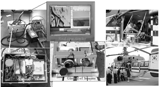
(3) Development of PKNU3: A small-format, multi-spectral, aerial photographic system. band of each CCD, and the sensitivity of the thermal. et al., 2004), an 18% reflective Kodak grey card was. infrared sensor for acquiring more accurate images. used as a reflectance standard to calibrate the camera. before actual flights. Few studies in current literatures. data for variations in incoming solar radiation.. discuss the correction of lens distortion in digital cameras. Jeong and Kim (2002) performed a related study that developed a program to correct the lens. 2. Materials and Methods. distortion of CCD cameras for mobile mapping systems. Mason et al. (1997) and Fraser et al. (1997) discussed lens distortion in their studies on the possibility of. 1) Chronological table of this study. generating a digital map of a small area using the Kodak. This study was initiated in January 2004. The field. DCS460 camera. In a study using color infrared (CIR). study, supported by the Ministry of Maritime Affairs. aerial photos based on ground-truth data to measure the. and Fisheries and the Korea Environmental Institute,. amount of chlorophyll on an exposed mudflat (Murphy. was completed with the second aerial photographic test. Table 1. Chronology of this study.. Date Date 1/2004 3/2004 3-7/2004 5/2004 5-9/2004 6-9/2004 7-8/2004 9/9/2004 9/14/2004. Contents Contents Investigation of native and foreign references Introduction of Redlake MS 4000 multi-spectral sensor Development of the data storage system Evaluation of the possibility of using PKNU3 onboard helicopters Manufacture of gimbals for sensors Connecting cable between sensors and data storage system Geometric and radiometric corrections of sensors First aerial photographic test Second aerial photographic test. Purpose Purpose Collect materials for development of the system Purchase equipment for the study Store still and moving pictures System development and safety Prevention of vibration onboard helicopter The pursuit of safety and convenience Evaluation of sensor characteristics Estimation of system’s fundamental capacity Possibility of high-volume photography with multi-spectral data. Fig. 1. Multi-spectral aerial photographic system and platform.. –339–.
(4) Korean Journal of Remote Sensing, Vol.20, No.5, 2004. in September 2004. The objectives of each test are. in this study senses the energy of the 7~14 mm. shown in Table 1.. wavelength as still and moving pictures and displays them through an LCD viewer. The distribution of the. 2) PKNU3 multi-spectral aerial photographic system. thermal energy in images can be displayed through the use of five colors (red, orange, yellow, green, and blue),. The PKNU3 system consists of a sensor array, a data. and temperatures can be shown in terms of brightness. storage system, and a platform (Fig. 1). The sensor. values. This camera was fitted with a Raytheon 50-mm. portion uses a Redlake MS 4000 (Redlake, San Diego,. F-1 lens. These two cameras (Redlake MS 4000 and. CA) multi-spectral camera and a Raytheon IRPro. Raytheon IRPro) were mounted on the gimbals that. thermal IR camera, which are both supported by. were specially designed to prevent platform vibration. gimbals to compensate for vibrations of the platform and. and to allow a wide range of adjustments of the. to allow for adjustments of the photographic angle. The. photographic angle. While the MS 4000 has autofocus,. data storage system is composed of an MPEG board,. the thermal IR camera does not; therefore, a separate. which can compress and transfer moving pictures as. unit was added to the gimbals/camera assembly to focus. high quality images in real time, and two computers,. the thermal IR camera remotely.. each with an 80-gigabyte memory capacity for data (2) Data storage system. storage. Helicopters were chosen as the aerial platform. A high-capacity data storage system is necessary to. over fixed-wing aircraft because they can rotate 360°. record the volumes of images because of the 1-s data. and fly at low speeds.. storage time of the MS 4000. Two compact computers. (1) Sensor portion. were implemented for the data storage system, each with. The PKNU2 system had drawbacks in its ability to. a storage capacity of 80 gigabytes and a 12-volt power. obtain composite, four-band images of any particular. supply. The two computers were tightly packaged in a. target area because the tasks of photographing the color. special case that insulated them from the vibration of a. and near-infrared images were divided between the. helicopter platform. To further reduce vibration, a. separate Kodak DCS 460 color and infrared cameras,. wiring harness was used that consolidated every. respectively. In addition, it was difficult to control the. connector between the sensor components and the data. minimum overlap rate (60%) owing to the 12-s storage. storage system into one thick cable.. delay. The Redlake MS 4000 sensor was introduced to overcome these drawbacks as well as to provide the. (3) GPS. capability of obtaining moving picture data.. A technique to acquire the exterior orientation. The Redlake MS 4000 sensor is a triple-CCD camera. parameters directly through combining several sensors. that can simultaneously take images in the R, G, B, and. in aerial reconnaissance aircraft was recently developed. IR bands, thus producing RGB and CIR images of the. by Ackermann (1993). GPS photogrammetry and. target area at 1600×1200 pixels (7.4 mm per pixel). The. GPS/INS photogrammetry allows the acquisition of. light sensitivity of the camera lens is controlled by using. exterior orientation parameters with only the use of a. gain values and an electronic shutter. The camera was. minimum of ground control points. The ground control. fitted with a Nikkon F-mount, 20-mm F2.8 rectillinear. process could even be completely skipped with a. lens. The Raytheon IRPro thermal infrared camera used. 30~50% reduction of the total cartography cost (Park et. –340–.
(5) Development of PKNU3: A small-format, multi-spectral, aerial photographic system. al., 2004). Various applications in GIS, airborne remote. Table 2. Precision.. sensing, and resource mapping often require data capture in fully digital form, with sufficient accuracy, speed, and cost-effectiveness. Therefore, integrated. Image precision. X (pixel) Y (pixel ) RMSE. Before correction for lens distortion 0.9374 0.8530 0.9195 After correction for lens distortion 0.6789 0.4936 0.5736. digital image acquisition and navigation systems have been developed for such applications (Cramer et al.,. The lens distortions were computed by comparing the. 1997; Mostafa et al., 1997; Toth and Grejner-. ground coordinates (reference) surveyed by theodolite. Brzezinska, 1998).. with the converted coordinates from the pixel numbers. In this research, a GPS antenna was included in. on the image of the panel in this paper. The lens. PKNU3 to compute the flight course, flight velocity, and. distortion was evaluated by using Eq. (1) with the. altitude of an aerial platform, as well as to provide the. following coefficients: K0 = 6.4817200e-3, K1 = -. three-dimensional coordinates (x, y, z) of each exposure. 4.4270500e-4 and K2 = 3.9596100e-6. Dr = k0r + k1r3 + k2r5 +…+ knr2n-1. location and a kappa value(K) among the rotation angles (w, f, K) of the platform for exterior orientation.. (1). where Dr is the radial distortion, r: is the radial distance, k0 through kn are the coefficients of radial distortion,. 3) Calibration and correction of sensors Prior to obtaining data from aerial photography, the sensor was calibrated to ensure that geometric and radiometric distortions of PKNU3 system itself are excluded.. and u is the variation. The image coordinate (x, y) corrections for the radial lens distortion were calculated from Eq. (2). The precision of x and y and the root mean square error (RMSE) of the image before and after the correction for. (1) Geometric correction of a multi-spectral. the lens distortion are shown in Table 2. x = x - x Dg, y = y - y Dg g g. camera (RGB/CIR MS 4000 sensor). Camera lens distortion resulting from the geometric structure of a lens is divided into radial distortion and tangential distortion. Tangential distortion is generally of much less consequence than radial distortion and can often be disregarded entirely; therefore, in this investigation, we performed calibration and correction only for radial distortion according to the following method.. (2). To obtain as little as 0.57~0.92 pixel lens distortion, we used only the central part of a CCD, which represents 12% of the available photographic area, as this area has the least lens distortion. It was possible to obtain images geometrically with a lens distortion of less than 1 pixel in size through calibration of the Redlake MS 4000 sensor for lens distortion.. A panel composed of 121 GCPs at regular intervals (2) Radiometric correction of the multi-spectral. was surveyed using a theodolite for correcting the radial. camera (RGB/CIR MS 4000 sensor). lens distortion, and an image of the panel was taken with the MS 4000 sensor. The ground coordinates (x, y, z). The measurements made by the multi-spectral sensor. were calculated using the horizontal angle (HA), vertical. must be calibrated with the spectrometer measurements of. angle (VA), and slope distance (SA) as surveyed by. the energy emitted and reflected by an object.. theodolite; the radial distance of ground coordinates, the. Radiometric corrections should be conducted to obtain the. radial distance of an image (r), and the radial distortion. actual intensity of solar radiant energy and reflectance.. (Dr) were computed.. The ability of the MS 4000 to photograph multi-spectrally –341–.
(6) Korean Journal of Remote Sensing, Vol.20, No.5, 2004. Fig. 2. Macbeth Color Checker & Bayer mosaic patterns of pixel filters & MS 4000 RGB/CIR configuration (from left).. was evaluated by verification of the radiometric. where Ll = spectral radiance at the sensor’s aperture. distortion. To compare and analyze between the ground-. (W/m2·sr·mm), QCAL = the quantized calibrated. truthing data and pixel values on the image, the Macbeth. pixel value in digital number (DN), LMIN l = the. Color Checker (GretagMacbeth Corp., New Windsor,. spectral radiance scaled to QCALMIN, LMAXl = the. NY; Fig. 2) was used; the results are shown in Table 3.. spectral radiance scaled to QCALMAX, QCALMIN =. The correlations between the brightness values on the. the minimum quantized calibrated pixel value. image and the measured solar radiant energy were. (corresponding to LMINl) in DN, QCALMAX = the. analyzed at different f-stops (2.8, 8, 11, 16) and exposure. maximum quantized calibrated pixel value. times to determine the maximum and minimum. (corresponding to LMAXl) in DN).. quantized calibrated pixel values (QCAL; effective. The gradients (Red: 8324.9, Green: 6921.8, Blue:. sensed range of the MS 4000 sensor). The effective. 4773.1) in Fig.3 are the radiant energy to the spectral. QCALs were then converted to spectral radiance at the. radiance. The more gradient increases, the less. sensor’s aperture by following Eq. (3), to compare them. sensitivity of CCD decreases. Hence, the sensitivity of a. to the ground-truthed values of radiant energy.. CCD for the red band was inferior to that of the others. It. L l = ((LMAX l - LMIN l )/(QCALMAXQCALMIN))×(QCAL-QCALMIN) + LMINl (3). is considered because a monochrome CCD sensor acquires the red plane at full resolution while it senses. Fig. 3. Correlations between spectral radiance in effective sensed range and radiant energy & Effective sensed range of MS 4000 sensor.. –342–.
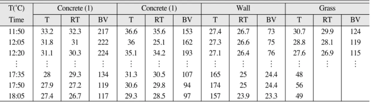
(7) Development of PKNU3: A small-format, multi-spectral, aerial photographic system. Table 3. Radiometric correction in each band (RGB).. Color Color Darkskin Lightskin Bluesky Foliage Blueflower Bluishgreen Moderatered Purple Yellowgre Orangeyellow Blue Green Red Yellow Magenta Cyan White Netual8 Netua6.5 Netua5 Netua3.5 Black Average. Correlation factor (CF) B G R 0.67 0.62 0.64 1.37 0.35 0.35 0.28 0.67 0.24 0.16 0.95 0.16 0.24 0.13 0.22 0.74 0.85 1.41 0.83 1.06 1.00 0.39 0.61. 0.50 0.41 0.41 0.97 0.20 0.25 0.14 0.29 0.79 0.25 0.32 0.31 0.11 0.40 0.08 0.46 0.71 0.94 0.55 0.84 0.68 0.18 0.45. 1.70 1.17 1.79 3.49 0.56 0.69 0.65 1.24 1.36 0.81 1.39 0.70 0.84 0.80 0.41 1.43 0.68 1.63 1.39 2.62 2.28 0.57 1.28. reflectance Spectral radiance at each band Groundtarget targetspectral spectral reflectance RGB pixel values Ground B G R B G R B G R 42 61 33 11 12 22 6550.54 5910.4 11653.6 131 160 89 32 26 41 18476.6 13292.9 21233.9 144 125 30 36 20 21 20463.2 10117.7 11053.4 56 95 19 30 36 26 16859.8 17356.4 13308.1 154 137 59 21 11 13 12123.7 5816.27 6514.9 155 183 37 21 18 10 12289.5 8728.59 5310.26 74 88 98 8 5 25 4720.16 2504.16 12872.1 69 52 33 18 6 16 10473.6 2937.26 8314.75 118 174 60 11 54 32 6777.2 26723.4 17053.2 81 181 95 5 18 30 2970.86 8971.79 15656.9 116 55 11 43 7 6 23167.3 3931.41 3387.36 93 150 22 6 18 6 3487.69 9313.34 3067.96 32 47 109 3 2 36 1918.06 1284.68 18662.5 95 164 109 5 26 34 2922.34 12926 17714.1 128 102 118 11 3 19 6146.13 1685.76 9997.59 173 150 16 50 27 9 28686.5 13656.6 4594.45 180 173 177 60 48 47 34644.5 24648.8 24497.8 154 180 97 85 66 62 48610.5 33959.9 32490.3 145 171 64 47 37 35 27061.8 18899.5 18289.7 115 125 37 48 41 38 27506.9 20790.7 20048.2 64 71 19 25 19 17 14039.2 9760.06 9022.75 26 29 9 4 2 2 2380.63 994.472 1169.23. the green (50%) and blue (25%) bands on the same. camera lens in the G and B bands and the R band,. CCD with a Bayer pattern as shown in Fig.2 to balance. respectively.. on R, G, and B sensitivity.. (3) Evaluation of characteristics of thermal. The calibration between the measured RGB. infrared sensor. reflectance of the color chart and the RGB values of the. If the emissivity (e) of an object is known, the total. image (i.e., the radiometric correction) was performed by calculating the correlation factor (CF) values from Eq. (4). CF = Ground target spectral reflectance / (RGB values/255). (4). The RGB sensitivity of the sensor was calculated using CF values (Ron Graham et al., 2002). According to the CF values, the MS 4000 was more sensitive for the G/B bands than for the R band. To maintain a proper. spectral radiant flux of an actual object can be calculated by modifying the Stefan-Bolzmann’s law (Mb = sTkin4) as applied to a black body. The following Eq. (5) takes into account the temperature and emissivity of an object for an accurate comparison between the radiant flux and the values reported on the thermal IR sensor (Chae Hyo Seog et al., 2002). Mr = eTkin4. balance among the R, G, and B bands of an image, the. (5). gain value was adjusted to increase or decrease the. The thermal infrared sensor generally reports the. response to the light reaching the CCD through the. outward radiant temperature (Krad) of an object as. –343–.
(8) Korean Journal of Remote Sensing, Vol.20, No.5, 2004. Table 4. Surveyed temperatures, radiant temperatures, and brightness values.. T(˚C) Time. T. 11:50 12:05 12:20 ⋯ 17:35 17:50 18:05. 33.2 31.8 31.1 ⋯ 28 27.9 27.4. Concrete (1) RT BV 32.3 31 30.3 ⋯ 29.3 27.2 26.7. 217 222 224 ⋯ 134 119 117. T 36.6 36 35.1 ⋯ 31.3 30.6 29.3. Concrete (1) RT BV 35.6 25.1 34.2 ⋯ 30.5 29.8 28.5. 153 162 193 ⋯ 107 94 97. T. Wall RT. BV. T. 27.4 27.3 27.1 ⋯ 165 174 157. 26.7 26.6 26.4 ⋯ 25 25 23.9. 73 75 76 ⋯ 24.4 24.4 23.3. 30.7 28.8 27.6 ⋯ 48 56 49. Grass RT. BV. 29.9 28.1 26.9 ⋯. 124 119 115 ⋯. opposed to the temperature (Tkin). The relationship. capabilities of PKNU3. An aerial platform (helicopter). between the radiant temperature input of an object on a. equipped with PKNU3 left the National Maritime Police. 1/4. sensor and the temperature is Krad = e Tkin. Therefore,. at Kimhae Airport at 24 min and 27 s past 2:00 PM and. the radiant temperature was calculated for each object. completed its flight plan at 48 min, 47 s past 3:00 PM on. with regard to emissivity in order to analyze the. September 9, 2004. According to the analysis of the recorded GPS data,. correlation with brightness values for an image, as. the altitude of the first flight was approximately between. shown in Table 4. The correlation coefficients between the outward. the minimum mean sea level (MSL) of 100 m and the. radiant temperature with regard to an object’s emissivity. maximum of 450 m with a maximum flying speed of. and the sensitivity of thermal IR sensor for each object. 200 km/h. We are unable to provide exterior orientation. were as high as 0.834 on concrete, 0.889 on a wall, and. using the GPS data for this test because the GPS. 0.725 on grass.. receiver was erroneously set to a 20-s data acquisition interval instead of the specified 1-s interval. Pictures taken in the first test were underexposed as a. 3. Results. result of cloudy and rainy weather and a lack of radiation intensity. Many images were out of focus as a result of miscalculation of an appropriate exposure time,. 1) First aerial photography test. because the helicopter’s speed was faster than the. The first test was an evaluation of the essential. Flight course (1st: red line, 2nd: blue line). anticipated 100 km/h. Moreover, it was difficult to. Change of 1st flight altitude (X:Julian second, Y:Mean Sea Level(MSL)) Fig. 4. First flight course, altitude, and velocity.. –344–. Change of 1st flight velocity (X:Julian second, Y:velocity(km/s)).
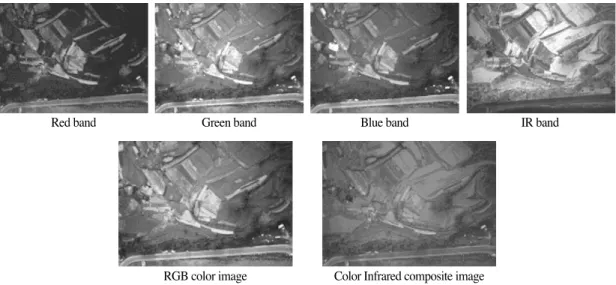
(9) Development of PKNU3: A small-format, multi-spectral, aerial photographic system. Red band. Green band. Blue band. RGB color image. IR band. Color Infrared composite image. Fig. 5. Still photographs (four-band).. maintain the proper balance among the sensitivities of. 25 min and 30 s past 3:00 PM at the same place, after. the R, G, B, and IR bands for each CCD sensor because. flying over Geojedo, Tongyoung, Gaduckdo, and the. a lack of radiation intensity made control of the gain. port of Daebyun. According to the GPS receiver data,. value difficult.. the flight altitude was between 100 and 400 m, and the. As a result of the first test, 278 sheets (7510 Kb each. flying speed was between 100 and 220 km/h (Fig. 6).. = 1.96 GB) of four-band still pictures in BSQ format, 72. PKNU3 took 6200 sheets (7510 Kb each = 46.56. min of moving color pictures (722 Mb), and 2.4 GB of. GB) of still pictures, 108 min of moving color pictures. moving thermal infrared pictures were obtained.. (4.16 GB), and 4.3 GB of moving thermal infrared pictures during the flight time of 1 h and 45 min. The. 2) Second aerial photography test. photographic area per image sheet was 0.022km2. Second test evaluated the capability of PKNU3 to provide high-volume multi-spectral photography. The. (0.17km×0.13km), and the spatial resolution was 0.11 m as a result of the low altitude.. second flight began at 19 min and 40 s before 2:00 PM. The images with overlap rates of 60-70% were. at Dalmaji Hill Airfield, Haeundae, Busan, and finished. obtained by automatically storing data at 1-s intervals.. Flight course (1st: red line, 2nd: blue line). Change of 2nd flight altitude (X:Julian second, Y:Mean Sea Level(MSL)). Change of 2nd flight velocity (X:Julian second, Y:velocity(km/s)). Fig. 6. Second flight course, altitude, and velocity.. –345–.
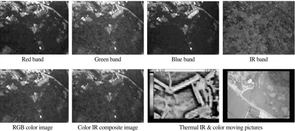
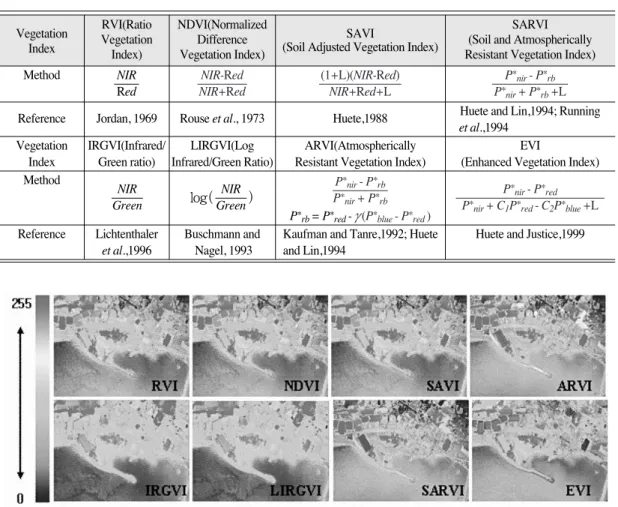
(10) Korean Journal of Remote Sensing, Vol.20, No.5, 2004. Red band. Green band. Blue band. RGB color image. Color IR composite image. IR band. Thermal IR & color moving pictures. Fig. 7. Results of the second flight: Still photographs (four-band), RGB, and CIR images, and thermal IR, color moving pictures.. Table 5. Camera attributes: x, y, z, and omega (w), phi (f), kappa (k).. time. x. y. z. W. f. k. 14:30:31 14:30:32 14:30:33 14:30:34 14:30:35 ⋯ 14:38:09 14:38:10 14:38:11. 148233 148223 148211 148198 148183 ⋯ 151429 151460 151491. 143953 143976 143999 144020 144042 ⋯ 155238 155257 155276. 269 271 272 274 275 ⋯ 303 301 299. 22 22 22 22 22 ⋯ 22 22 22. 17 17 17 17 17 ⋯ 17 17 17. -342 -338 -334 -331 -328 ⋯ -65 -65 -63. The attributes of sensor shown in Table 5 include the. compare with the spectral indices, therefore, the. coordinates and rotation values of the platform at each. practicality of PKNU3 was evaluated by an inductive. exposure station. The gain values and exposure times for. method analyzing the coefficients among the spectral. each band to control the response of the CCD to the light. signatures of chlorophyll images including NDVI, RVI,. passing through the lens were 3 in G/B bands and 6 in R. SAVI, and etc., which have been already used as a way. and NIR bands, and 4 milliseconds for every band.. to extract the related information with covered vegetation on the earth from satellite images and aerial. 3) Application of results. photographs for over 30 years. The study of Murphy et. Several vegetation indices were applied to imageries. al., which described a field-based method to estimate. taken by PKNU 3 for evaluating the utility of them as a. chlorophyll using digital color-infrared photograph. data for Environmental remote sensing. The usefulness. taken by Duncantech 3-band CIR camera, having the. of remotely sensed data for any application is dependent. same spectral configuration as MS4000 sensor, supports. upon the acquisition of appropriate ground-truth data.. this reasoning by induction (Table 6).. However we didn’t measure in situ chlorophyll to –346–. The images applied each index are displayed as RGB.
(11) Development of PKNU3: A small-format, multi-spectral, aerial photographic system. Table 6. Vegetation indices used in this study.. Vegetation Vegetation Index Index. RVI(Ratio NDVI(Normalized SAVI SAVI Vegetation Difference Vegetation Index) Difference Vegetation (Soil Adjusted Vegetation Index) (Soil Adjusted Vegetation Index) Index) Vegetation Index)Index). Method. NIR Red. NIR-Red NIR+Red. (1+L)(NIR-Red) NIR+Red+L. Reference. Jordan, 1969. Rouse et al., 1973. Huete,1988. Vegetation Index Method. Reference. IRGVI(Infrared/ LIRGVI(Log Green ratio) Infrared/Green Ratio) NIR Green. log( Green ). NIR. Lichtenthaler et al.,1996. Buschmann and Nagel, 1993. ARVI(Atmospherically Resistant Vegetation Index) P*nir - P*rb P*nir + P*rb P*rb = P*red - g (P*blue - P*red ) Kaufman and Tanre,1992; Huete and Lin,1994. SARVI (Soil and Atmospherically Resistant Resistant Vegetation Vegetation Index) Index) P*nir - P*rb P*nir + P*rb +L Huete and Lin,1994; Running et al.,1994 EVI (Enhanced Vegetation Index) P*nir - P*red P*nir + C1P*red - C2P*blue +L Huete and Justice,1999. Fig. 8. Images of each vegetation index derived from PKNU 3 photos. Table 7. Correlation coefficients among vegetation indices applied to imageries. RVI NDVI SAVI IRGVI LIRGVI ARVI SARVI EVI. RVI. NDVI. SAVI. IRGVI. LIRGVI. ARVI. SARVI. EVI. 1 0.99 0.99 0.70 0.65 0.82 0.82 0.47. 0.99 1 1 0.71 0.67 0.80 0.80 0.47. 0.99 1 1 0.71 0.67 0.80 0.80 0.47. 0.70 0.71 0.71 1 1 0.22 0.22 0.71. 0.65 0.67 0.67 1 1 0.22 0.22 0.56. 0.82 0.80 0.80 0.22 0.22 1 1 -0.08. 0.82 0.80 0.80 0.22 0.22 1 1 -0.08. 0.47 0.47 0.47 0.71 0.56 -0.08 -0.08 1. color of the range of 0-255 in Fig. 8.. The correlation coefficients in RVI, NDVI and SAVI. The mean values of spectral signatures in imagery. indices are high (Table 7) same as the result of Murphy. were calculated to analyze correlation among imageries. et al. which resulted in a modest improvement in the. applied vegetation indices in Table 7.. linear fit between the measure of chlorophyll and the –347–.
(12) 100 90 80 70 60 50 40 30 20 10 0 -0.1. ChlorophyII(mg, cm). ChlorophyII(mg, dry sediment). Korean Journal of Remote Sensing, Vol.20, No.5, 2004. 0.0. 0.1. 0.2. 0.3. 0.4. 22 20 18 16 14 12 10 8 6 4 2 0 -0.1. 0.0. 0.1. 0.2. 0.3. 0.4. Fig. 9. Relationship between area- and weight-normalized chlorophyll and SAVI. (a) Weight-normalized chlorophyll and SAVI (R2=0.31, P<0.01, n=61). (b) Area-normalized chlorophyll and SAVI (R2=0.50, P<0.01, n=61). <The source of figure: R. J. Murphy et al., 2004>. RVI, NDVI and SAVI indices(Fig.9). The distribution. of 60-70% using the automatic 1-s interval data. of chlorophyll in the RVI and NDVI images exhibits a. recording time is now possible. Third, the thermal IR sensor’s lack of autofocus has. spatial pattern almost identical to that observed in the. been mitigated by the successful implementation of a. SAVI image (Murphy et al., 2004). According to Murphy et al., the field-based CIR photography will provide a useful tool for the non-. remote focus-control system that is installed in the gimbals/camera assembly.. destructive determination of benthic chlorophyll.. Fourth, to limit the lens distortion to as little as 0.57-. Therefore, it is considered that the PKNU 3 system can. 0.92 pixels, only the central 12% of the available. be used as a method of Environmental remote sensing.. photographic area, where lens distortion is least, is used. Fifth, to maintain the proper balance among the R, G, and B bands of an image, the gain values are lowered for. 4. Conclusions. the G/B band and raised for the R band to adjust the responses to the light reaching the CCD through the. As of September 2004, the PKNU3 development. camera lens.. schedule has reached the second phase of testing.. Sixth, the sensitivity of CCD for the red band is. Various experiments and tasks have been conducted to. inferior to that for other bands because a monochrome. improve this system, and the following have been. CCD sensor acquires the red plane at full resolution. achieved.. whereas it senses the green and blue bands on the same. First, a multi-spectral, aerial photographic system has. CCD with a Bayer pattern.. been created that, at its core, consists of a sensor capable. Seventh, the correlation coefficients between the. of taking R, G, B, and IR images simultaneously,. outward radiant temperature regarding an object’s. immediately producing a composite RGB and CIR. emissivity and the sensitivity of the thermal IR sensor. image of a target area coupled with a thermal infrared. for each object are as high as 0.834 for concrete, 0.889. image.. for a wall, and 0.725 for grass.. Second, using the integrated data storage system,. Eighth, it was determined that the images taken. high-volume photography on long-distance flights as. during the first flight were out of focus owing to a. well as the ability to obtain images with an overlap rate. miscalculation of the appropriate exposure time. –348–.
(13) Development of PKNU3: A small-format, multi-spectral, aerial photographic system. (resulting from a lack of synchronization between the. ISPRS Journal of Photogrammetry and Remote. velocity of the aerial platform and the exposure. Sensing, 52(4): 149-159.. calculations) and to a difficulty in maintaining a proper. Cramer, M., D. Stallmann, and N. Haala, 1997. High. balance among the sensitivities of the R, G, B, and IR. precision georeferencing using GPS/INS and. bands for each CCD sensor, which was attributable to. image matching, Proc. International Symposium. inaccurate gain values as a result of the low-intensity of. on Kinematic Systems in Geodesy, Geomatics. radiation.. and Navigation, Banff, Canada, pp.453- 462.. Ninth, determination of appropriate exposure times. Cramer, M., D. Stallmann, and N. Haala, , 2000. Direct. and gain values during the second test were successfully. Georereferencing Using GPS/Inertial Exterior. accomplished, and the coordinates and rotation value. Orientations for Photogrammetric Applications,. (only kappa value) of the platform at each exposure. ISPRS Vol. XXXIII Part B3/1, pp.198-206.. station were computed from the processed GPS data.. Ackermann, F. and H. Schade, 1993. Application of GPS. Further study is warranted to enhance the system with. for Aerial Triangulation, Photogrammetiric. the addition of gyroscopic and IMU units for obtaining. Engineering & Remote Sensing, 59(11): 18-39.. omega and phi values and to verify the data and. Hagerthey, S. E., D. M. Paterson, and J. Kromkamp,. calibration procedures of the system to produce strips. 2002. Monitoring estuarine ecosystems: the Eden. automatically.. Estuary and the BIOPTIS programme. Estuarine. Tenth, the PKNU 3 data will be used as a useful tool. and Coastal Sciences Association, 2003. Coastal. for Environmental remote sensing. We need to measure. Zone Topics, 5. The Estuaries and Coasts of. ground-truth chlorophyll directly in the study area and. North-East Scotland. Aberdeen, Estuarine and Coastal Sciences Association, pp.89-97.. compare with the other indices for proving the utility of. Hakvoort, J. H. M., M. Heineke, K. Heyman, H. Kuhl,. PKNU 3 system in the future study.. R. Riethmuller, and G. Witte, 1998. A basis for mapping the erodibility of tidal flats by optical. Acknowledgements. remote sensing. Marine and Freshwater Research, 49: 867-873.. We express our gratitude to the Pukyong National. Huete, A. R., 1996. A Soil-adjusted Vegetation. University, the Ministry of Maritime Affairs and. Index(SAVI), Remote sensing of Environment,. Fisheries, and the Korea Environmental Institute for. 25: 295-309. Heute, A. and C. Justice, 1999. MODIS Vegetation Index. their support of this study.. (MOD 13) Algorithm Theoretical Basis Document, Greenbelt: NASA Goddard Space Flight Center,. References. http://modarch.gsfc.nasa.gov/MODIS/LAND/ #vegetation indices, 129p.. Buschmann, C. and E. Nagel, 1993. In vivo. Heute, A. F. and H. Q. Liu, 1994. An Error and. spectroscopy of internal optics of leaves as basis. Sensitivity Analysis of the Atmospheric-and. for remote sensing of vegetation, International. Solid-Collecting Variants of the Normalized. Journal of Remote Sensing, 14 (4): 711-722.. Difference Vegetation Index for the MODIS-. Clive S. Fraser, 1997. Digital camera self-calibration, –349–. EOS, IEEE Transactions on Geoscience and.
(14) Korean Journal of Remote Sensing, Vol.20, No.5, 2004. Remote Sensing, 32(4): 897-905.. terrain modeling, Geomorphology, 29: 77-92.. Huete, A. R., G. Hua, J. Qi, A. Chehbouni and W. J.. Mostafa, M. M. R. and K. P. Schwarz, 2001. Digital image. Van Leeuwem, 1992. .Normalization of. georeferencing from a multiple camera system by. Multidirectional Red and Near-Infrared. GPS/INS, ISPRS Journal of Photogrammetry &. Reflectances with the SAVI,. Remote Sensing of. Remote Sensing, 5(1): 1-12.. Environment, 40: 1-20.. Mostafa, M. M. R., K. P. Schwarz, and P. Gong, 1997. A. Jeong, D-H, and B-G. Kim, 2002. Surveying and Geo-. fully digital system for airborne mapping, Proc.. Spatial Information Engineering: Lens. International Symposium on Kinematic Systems. Distortion Correction for CCD Camera using. in Geodesy, Geomatics, and Navigation, Banff,. Projective Transformation Method, The Korean society of Civil engineers collected papers D,. Alberta, Canada, pp.463-471. Nüsslein, S., A. Greune, H. Adler, A. Troycke, G. Faisst, S.. 22(5): 995-1001.. Reimeier, and R. Dietrich, 1997. Totholzflächen. Murphy, R. J., T. J. Tolhurst, M. G. Chapman, and A. J.. und Waldstrukturdaten im Nationalpark. Underwood, 2004. Estimation of surface. Bayerischer Wald (1996/1997), Bayerische. chlorophyll on an exposed mudflat using digital. Landesanstalt fur Wald und Forstwirtschaft,. colour-infrared (CIR) photography, Estuarine,. Dfreising.. Coastal and Shelf Science, 59: 625-638.. Park, W-Y, K-W Lee, J-O Lee, and G-U Jeong, 2004,. Jensen J. R., H-S Chae, G-E Kim, S-J Kim, Y-S Kim,. Block Adjustment with GPS/INS in Aerial. K-S Lee, K-S Cho, and M-H Jo, 2002,. Photogrammetry, Journal of the Korean Society. Environment Remote Sensing, Sigma Press,. of Surveying, Geodesy, Photogrammetry, and. Prentice Hall, pp.255-297, 381-386.. Cartography, 22(3): 285-291.. Jordan, C. F., 1969. Derivation of leaf area index from. Riethmuller, R., J. H. M. Hakvoort, M. Heineke, K.. quality of light on the forest floor, Ecology, 50:. Heymann, H. Kuhl, and G. Witte, 1998.. 663-666.. Relating erosion shear stress to tidal flat surface. Koch, B., D. Münch, T. Pröbsting, 1998. Totholz als. colour. In: Black, K.S., Paterson, D.M., Cramp,. ökosystemare Eingangsgrösse, In: Fischer, A.. A. (Eds.), Sedimentary Processes in the. (Ed.), Die Entwicklung von Wald-Biozö nosen. Intertidal Zone. Special Publications 139.. nach Sturmwurf. Landsberg, Baden-Wü. Geological Society, London, pp.283-293.. rttemberg, pp.64-73.. Graham R. and A. Koh, 2002. Digital Aerial Survey Theory. L. Shukai, 1992. Analysis of Remote Sensing of Global Environment and Resources, Surveying and. and Practice, Whittles Publishing, pp.52-121. Rouse, J. W., R. H. Haas, J. A. Schell, and D. W. Deering,. Mapping Press, Beijing.. 1973. Monitoring vegetation systems in the great. Lichtenthaler, H. K., A. Gitelson, M. Lang, 1996. Non-. plains with ERTS, Third ERTS Symposium,. destructive determination of chlorophyll content. NASA SP-351, vol. 1, NASA, Washington DC,. of leaves of a green and an aurea mutant of. pp.309-317.. tobacco by reflectance measurements, Journal. Running, S. W., C. O. Justice, V. Solomonson, D. Hall, J.. of Plant Physiology, 148: 483-493.. Baker, Y. J. Kaufmann, A. H. Strahler, A. R.. Livingstone, D., J. Raper, and T. McCarthy, 1999. Integrating. Heute, J. P. Muller, V. Vanderbilt, Z. M. Wan, P.. aerial videography and digital photography with. Teillet, and D. Carneggie, 1994. Terrestrial. –350–.
(15) Development of PKNU3: A small-format, multi-spectral, aerial photographic system. Remote Sensing Science and Algorithms. mapping, ISPRS Journal of Photogrammetry &. Planned for EOS/MODIS, Int. Journal of Remote. Remote Sensing, 52(5): 202-214. Toth, C. and D. A. Grejner-Brzezinska, 1998.. Sensing, 15(17): 3587-3620.. ∨. Scherrer, H. U.,1993. Projekt zur flachenhaften. Performance analysis Z. of the airborne. Erfassung und Auswertung von Sturmschaden,. integrated mapping system AIMSe, Int. Z. Arch.. AFZ/Der Wald, 14: 712-714.. Photogr. Remote Sens., 32(2): 320-326.. Schmidtke, H., 1993. Die fraktale Geometrie von. ∨. G. J. C. Underwood, and J. Kromkamp, 1999. Primary. Sturmschaden-flächen im Wald, AFZ/Der. production. Wald, 14: 710-712.. microphytobenthos in estuaries. Advances in. Mason, S., H. Ruther, and J. Smit, 1997. Investigation of the Kodak DCS460 digital camera for small-area. –351–. by. phytoplankton. Ecological Research, 29: 93-153.. and.
(16) Korean Journal of Remote Sensing, Vol.20, No.5, 2004. –352–.
(17)
수치

+3
관련 문서
