To whom corresponding should be addressed.
30, Jangjeon-dong, Geumjeong-gu, Busan, 609-735 Tel : 051-510-2455 E-mail : [email protected]
Numerical
Numerical Numerical
Numerical Evaluation Evaluation Evaluation Evaluation of of of the of the the the Cooling Cooling Cooling Cooling Performance Performance Performance Performance of of of of a a a
a Core Core Core Core Catcher Catcher Catcher Catcher Test Test Test Test Facility Facility Facility Facility
Dong Hun Lee
*, Ik Kyu Park
**, Han Young Yoon
**, Kwang Soon Ha
**, Jae Jun Jeong
**
School of Mechanical Engineering, Pusan National University,
**
Korea Atomic Energy Research Institute (KAERI)
(Received 3 December 2012, Revised 11 March 2013, Accepted 11 March 2013) Abstract
Abstract Abstract Abstract
A core catcher is considered as a promising engineered system to stabilize the molten corium in the containment during a postulated severe accident in a nuclear power plant. Conceptually, the core catcher consists of a carbon steel body, sacrificial material, protection material, and engineered cooling channel. The cooling capacity of the engineered cooling channel should be guaranteed to remove the decay heat of the molten corium. The flow in ex-vessel core catcher is a combined problem of a two-phase flow in the engineered cooling channel and a single-phase natural circulation in the whole core catcher system. In this study, the analysis of the test facility for the core catcher using the CUPID code, which is a three-dimensional thermal-hydraulic code for the simulation of two-phase flows, was carried out to evaluate its cooling capacity.
Key words : core catcher, natural circulation, two-phase flow, CUPID code
1. Introduction
Nuclear power plants have various safety systems designed to prevent postulated accidents, to enhance the life time and economic benefit, and to increase public acceptance of the plants. Recently, a hypothetical severe accident, which is beyond design basis accident, is becoming a serious issue.
In the current generation of nuclear power plants, there might be a chance of a severe accident. Thus, many systems have been developed against severe accidents. In particular, these systems have adopted a passive concept to operate in the case of a station black out.
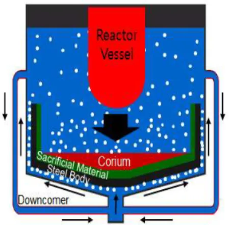
A core catcher for a next-generation advanced light water reactor has been developed to stabilize the molten corium by preventing the molten corium-concrete interaction in the reactor
containment during a severe accident. As schematically shown in Fig. 1, a core catcher consists of a carbon steel body, sacrificial material, protection material, and engineered cooling channel.
The molten corium discharged from a failure of the reactor vessel is collected inside the core catcher body. The sensible and decay heat of the molten corium are to be removed by the coolant channel placed on the external face of the core catcher body, where a two-phase natural circulation flow is developed [1]. The flow phenomena in the core catcher system are characterized by multi-dimensional two-phase flow behaviors with a weak driving force of the gravity. Therefore, a multi-dimensional analysis is required for investigating this natural circulation.
The multi-dimensional components of system
codes and some commercial CFD codes are not
applicable to practical two-phase flow problems
because of their physical and numerical limitations
Fig. 1. Schematic diagram of the core catcher.
for simulating complicated flows with drastic phase changes [2]. In this regard, the CUPID code is a promising tool for the analysis of the core catcher system. The CUPID code has been developed by KAERI for the analysis of transient, multi-dimensional, two-phase flows in nuclear reactor components [2]. The CUPID code adopts a two-fluid, three-field model for two-phase flow. The physical modeling and numerical solution method of the CUPID code put an emphasis on versatile and robust simulations of complicated two-phase flows. This is based on a practical need to overcome the shortcomings of existing CFD codes and the multi-dimensional component of system codes.
This paper presents a preliminary analysis of the core catcher experimental facility using the CUPID code, mainly focusing on the phenomena and the heat removal capability by the natural circulation of the two-phase flow of the core catcher.
2. Mathematical Model of CUPID Code
2-1 Governing Equations
To simulate a two-phase flow, CUPID adopts a transient two-fluid, three-field model. The three fields are a continuous liquid, droplets, and a vapor.
The governing equations of this model are similar to those of the time-averaged two-fluid model derived by Ishii and Hibiki [3]. The continuity,
momentum, and energy equations for the k-field are given by
k k k k k
k
ρ ) α ρ u
t (α + ∇ = Γ
∂
∂
(1)
) u u ρ (α u ρ
t α
k k k+ ∇ ⋅
k k k k∂
∂
k k k k eff k , k
k
P α µ u α ρ g S
α ∇ + ∇ ⋅ ∇ + +
−
= ( )
(2) )
u e ρ t (α
) e ρ (α
k k k k k
k
k
+ ∇ ⋅
∂
∂
k k k c , k k
k
k
P (α u ) α k T E
t
P α
− ∇⋅ +∇⋅ ∇ +∂
− ∂
= ( )
, (3) where α
k, ρ
k, u
k, P, Г
k, and e
kare the k-field volume fraction, density, velocity, pressure, interface mass transfer rate, and energy transfer rate, respectively. S
krepresents the interfacial momentum transfer due to a mass exchange, a drag force, and non-drag forces. E
kincludes the phase change, interfacial heat transfer, wall heat transfer, and volumetric heat source.
For a mathematical closure of the system of equations, constitutive relations and the equations of state are included.
To obtain numerical solutions, the finite volume method is applied to the two-fluid governing equations on unstructured grids. The solution algorithm of the CUPID code was originally developed from the semi-implicit method for a two-phase flow [4, 5] with some modifications for an application to unstructured non-staggered grids.
The method was further improved for enhanced robustness and accuracy [6].
2-2 Physical Models and Correlations
Some of the physical models and correlations relevant to the core catcher analysis are briefly introduced in this section.
In a two-phase flow, the interfacial momentum
and heat transfer strongly depend on the shape of
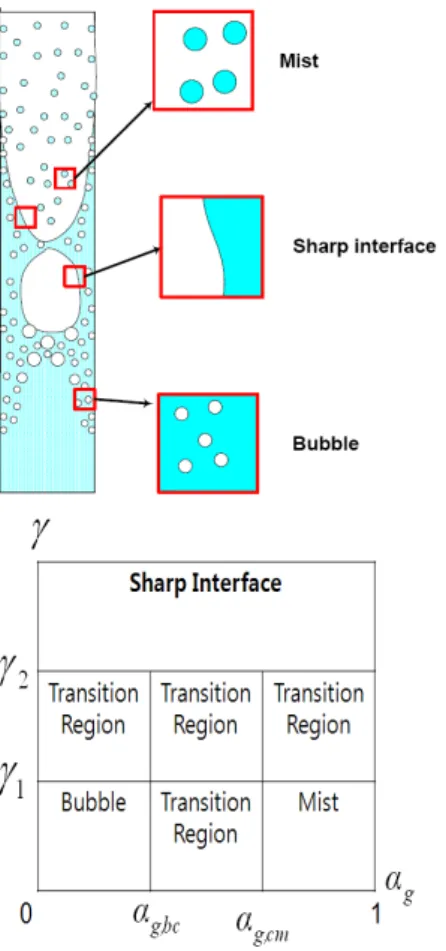
Fig. 2. Inter-phase surface topology concept.
. the liquid-vapor interface. To model local interface
structure of the two-phase flow, the inter-phase topology concept proposed by Tentner et al. [7] was employed in the CUPID code. They proposed the inter-phase surface topology map [8, 9]. Their works have attempted simulations of not only dispersed flows but also flows involving a local sharp interface, such as slug and annular-mist flows.
In the approach, three main types of local inter-phase surface topologies and the transitional regions are distinguished, as shown in Fig. 2. The main topologies are a bubbly flow, a mist flow, and a sharp interface topology. The transitional topologies are the overlapping regions of two or three main topologies. The topology in each mesh cell is determined by two parameters, a void
fraction,
g,and a void fraction difference, γ = δ ⋅ ∇ α
g[10]. Once the local topology is determined for each cell, the interfacial momentum and heat transfer models [2, 10] are calculated, depending on the topology of each cell.
In the CUPID, two models are available for the turbulent shear stress; one is the mixing length model and the other one is the standard k- ε model.
The effective viscosity of the continuous liquid phase can be calculated by the sum of the bubble effect viscosity. In the case of a bubbly two-phase flow, the effect of the bubble`s motion on the turbulence has been modeled as a function of the Sauter-mean bubble diameter and relative velocity, and is considered additionally [11]. The effective viscosity of the dispersed gas phase can be calculated by assuming the same kinematic viscosity of the liquid and gas.
In a subcooled boiling flow, the amount of vapor generation is computed by a wall heat flux partitioning model. The heat transfer from the wall consists of the surface quenching, q
q, evaporative heat transfer, q
e, and single-phase convection, q
c, which are explained as follows [12].
c e
q
q q
q
q
= + +, (4) (
w l)
f l p l l c w
q
t k c f A T T
q
−
= 2 ,
ρ
, 2π , (5)
lg g d
e
N f D h
q π ρ
=
3" 6
, (6)
(
w c)
c c
c
h A T T
q = − , (7)
) (
g,sat le
wall
h h
q
= −
Γ (8)
The wall vapor generation rate is calculated by
Eq. (8). Eq. (4) is a non-linear equation with an
unknown wall temperature, T
w. The equation can be
Fig. 3. Shematic diagram of the conceptual design of the prototype core catcher.
Fig. 4. Schematic diagram of the test facility.
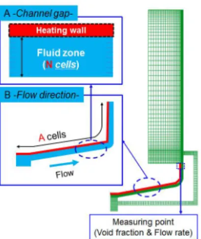
Fig. 5. Calculation domain and grid configurations for mesh sensitivity analysis : case A (channel gap), case B (flow direction).
solved by the Newton-Raphson method.
3. Analysis of the Core Catcher
3-1 The Test Facility for the Core Catcher The schematic diagram of the conceptual design of a prototype core catcher [13] is presented in Figs. 1 and 3. The core catcher has a rectangular shape with a dimension of 6 m x 16 m x 7 m.
To evaluate the core catcher cooling performance, KAERI has designed a test facility maintaining the thermal-hydraulic similarity with the prototype [13].
The schematic diagram of the test facility is shown in Fig. 4. It has been designed to simulate the right half of the prototype. The cooling channel of the core catcher has a gap size of 0.1 m and an angle
of inclination of 10 degrees [1]. The total length of the circulation loop from the cooling channel and the downcomer is about 10 m. A water tank with a dimension 1.5 m x 6.4 m is set up on the loop.
In the subsequent analysis, it is assumed that the tank is initially filled with water at a temperature of 97 °C. The top of the tank is open to a constant pressure boundary of 0.1 MPa. The heater block is modeled as a constant heat flux boundary. The heat flux from the molten corium is assumed to be 0.133 MW/m
2[13].
3-2 Mesh Sensitivity Analysis
To simulate the test facility using the CUPID code, a two-dimensional grid was adopted. It is noted that a two-dimensional approach was also applied for the design of the test facility.
At first, a based input was prepared, which is based on the wide range of experiences from the CUPID code validation activities [2]. Then, the mesh sensitivity analysis on the cooling channel was carried out as shown in Fig. 5:
(i) Case A is a sensitivity analysis on the channel
gap direction. 4, 6, 8, and 10 cells were used.
10 20 30 40
F lo w r a te ( k g /s )
N=4 N=6 N=8 N=10
Fig. 6. Case A (channel gap) : flow rate in the cooling channel.
10 20 30 40
F lo w r a te ( k g /s )
A=85 A=125 A=170
Fig. 7. Case B (flow direction) : flow rate in the cooling channel.
Fig. 8. Liquid velocity vector.
(a) (b)
Fig. 9. Contour : (a) pressure, and (b) temperature of liquid.
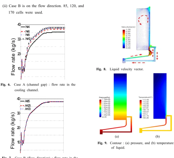
(ii) Case B is on the flow direction. 85, 120, and 170 cells were used.
Figs. 6 and 7 show the calculated mass flow rate at the cooling channel, which converges to a certain value by using finer meshes. The result of case A indicates that more than 10 meshes to the channel gap direction are sufficient. Meanwhile, the result of case B shows that 85 meshes are enough to avoid mesh effects as presented in Fig. 7.
Thus, the cooling channel was discretized into a grid of 10 meshes in the gap direction and 85 meshes in the flow direction. A total computation grid with 3224 cells was used for this calculation.
It is noted that the standard k-ε model was used in this analysis.
3-3 Calculation Results
A null-transient was calculated to reach a steady state for the conditions given in section 3-1. The steady-state velocity vector is shown in Fig. 8. The flow velocity near the heated wall is faster due to a high void fraction. It seems that a two-phase natural circulation flow along the cooling channel and the downcomer is reasonably simulated considering the flow path. Fig. 8 also shows that a natural circulation flow in the water tank is formed due to the heated water flow from the cooling channel.
The contours of liquid pressure and temperature
are shown in Fig. 9. The pressures are properly
Fig. 10. Void fraction.
0.04 0.08 0.12 0.16
V o id f ra c tio n
Fig. 11. Void fraction distribution of the channel outlet.
-1 0 1 2 3
S u b co o lin g(
oC )
At 440 seconds, a flashing occurs.
Fig. 12. Subcooling temperature of the water tank outlet.
Table 1. Comparison the analytical solution with the CUPID calculation.
Analytical solution
CUPID calculation Slip ratio(=u
g/u
l) 2.0 ~1.7 Mass flux(kg/m
2.s) 348.7 381.2 calculated according to the water height as depicted
in Fig. 9 (a). The temperature near the heated wall is higher than that in any other place, as shown in Fig. 9 (b). And the liquid temperature distribution is reasonably consistent with the liquid circulation in the tank. In the upper region of the tank, the liquid temperature is slightly greater than the saturation temperature at 440 seconds as presented in Fig. 12.
This resulted in a flashing, as shown in Fig. 10.
The steady-state void fraction distribution is shown in Fig. 10. Bubbles are generated at the heater block and move upwards to the water tank.
However, all bubbles are condensed in the subcooled water at the right bottom of the water tank. Thus, no bubbles enter the downcomer channel.
Fig. 11 shows the void fraction distribution
across the gap at the top of the heated channel. The void fraction is greater near the heated wall and gradually decreases, which is physically reasonable.
The flow rate at the downcomer is presented in Fig. 6. It shows that the circulation flow reaches a steady-state at the mass flow rate of 38.12 kg/s with a heat flux of 0.133 MW/m
2. The mass flow rate in this calculation is equivalent to a mass flux of 381.2 kg/m
2.s.
At present, no experimental data are available for
a comparison with the calculation results. Instead,
analytical solutions for the prototype were obtained
by a balance between the pressure drop and
hydrostatic head with some assumptions [14]. In the
analysis, the mass flux was evaluated to be of
348.7 kg/m
2.s with the assumption that the slip ratio
at the exit of the cooling channel is 2.0. The higher
slip ratio leads to a smaller void fraction, resulting
in a smaller driving force and, thus, a smaller flow
0.02 0.04 0.06 0.08
V o id f ra ct io n
H=4.4m H=5.4m H=6.4m
10 20 30 40 50
F lo w r a te ( kg /s )
H=4.4m H=5.4m H=6.4m
(a) Void fraction of the channel outlet
(b) Flow rate of the downcomer Fig. 13. Parametric study for the water tank height.
0.03 0.06 0.09 0.12 0.15
V o id f ra ct io n
Q=150kw/m2 Q=200kw/m2 Q=250kw/m2
0 20 40 60 80
F lo w r a te ( k g /s )
Q=150kw/m2 Q=200kw/m2 Q=250kw/m2