Estimations of the skew parameter in a skewed double power function distribution

Estimations of the skew parameter in a skewed double power function distribution

Jun-ho Kang ¹ · Chang-Soo Lee ²

1 Department of Special Physical Education, Kaya University

2 Department of Flight Operation, Kyungwoon University

Received 22 April 2013, revised 16 May 2013, accepted 3 June 2013

Abstract

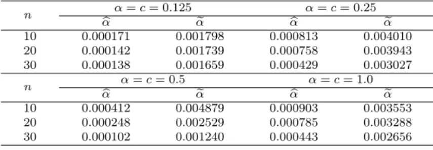
A skewed double power function distribution is defined by a double power function distribution. We shall evaluate the coefficient of the skewness of a skewed double power function distribution. We shall obtain an approximate maximum likelihood estimator (MLE) and a moment estimator (MME) of the skew parameter in the skewed double power function distribution, and compare simulated mean squared errors for those estimators. And we shall compare simulated MSEs of two proposed reliability estimators in two independent skewed double power function distributions with different skew parameters.

Keywords: Approximate MLE, moment estimator, reliability, right-tail probability, skewed double power function distribution, skewness.

1. Introduction

Many authors have studied estimations and characterizations of a double power func- tion distribution. Ali and Woo (2006) and Woo (2006) studied several skew -symmetric reflected distributions, which do not include some reflected distributions. Azzalini and Cap- itanio (1999) studied the multivariate skewed normal distribution and Woo (2007) studied the reliability in a half-triangle distribution and a skewed distribution. Balakrishnan and Cohen (1991) proposed the method of finding an approximate MLE for the scale parameter in several distributions. Han and Kang (2006) studied an approximate MLE of parameters in several distributions with censored samples. Son and Woo (2007) studied an approx- imate MLE in a skew-symmetric Laplace distribution Lee and Lee (2012) considered an approximate MLE in a weight exponential distribution. It is not easy for us to estimate the skew parameter in a skewed distribution, so we consider an approximate MLE of the skew parameter in a skewed double power function distribution.

In this paper, a skewed double power function distribution is defined by a double power function distribution. And we shall evaluate the coefficient of the skewness of a skewed double power function distribution. We shall obtain an approximate MLE and a moment

1

Associate professor, Department of Special Physical Education, Kaya University, Gimhae 621-748, Korea

2

Corresponding author : Associate professor, Department of Flight Operation, Kyungwoon University,

Gumi 730-850, Korea. E-mail : [email protected]

estimator of the skew parameter in the skewed double power function distribution and then compare simulated MSEs of those estimators. And we shall compare simulated MSEs of two proposed reliability estimators in independent skewed double power function distributions with different skew parameters. Finally, we shall introduce a skewed double power func- tion distribution generated by a double Weibull distribution and observe the skewness by evaluating its coefficient of the skewness.

2. A skewed double power function distribution

Let X and Y be independent and identically distributed random variables with the con- tinuous density function(pdf) f (x) = F ⁰ (x) which it is symmetric about the origin. Then for ^∀ α ∈ R ¹ ,

1

2 = P (X ≤ αY ) = Z ∞

−∞

f (t)F (αt)dt.

Hence, a skewed density function is given, as in Azzalini (1985), by :

f (z; α) ≡ 2f (z)F (αz). (2.1)

The density function f (z; α) becomes a skewed density of a random variable Z having the symmetric density and α is called the skew parameter of the density. Especially, if α = 0, then f (z; 0) becomes the original symmetric density.

From the skewed density function (2.1), the cumulative distribution function (cdf) of the skewed random variable Z with the density (2.1) is given, as in Azzalini (1985), by :

F (z; α) = 2 Z z

−∞

f (t)

Z α(t−θ)+θ

−∞

f (s)dsdt. (2.2)

2.1. Skewness of a skewed double power function distribution

The density function of a double power function random variable X is given, as in Johnson et al. (1994) by :

f (x) = θ|x| ^θ−1 /2, if |x| ≤ 1, θ > 0 and the cdf is given by :

F (x) = 1

2 (1 + sgn(x)|x| ^θ ), if |x| ≤ 1, where sgn(x) = n ₁ if x > 0

−1, if x < 0 .

Especially, if θ = 1, then a random variable X has an uniform distribution over (-1,1).

Also, if Y = − ln |X|, then Y has an exponential distribution with the mean 1/θ.

Define

α ^∗ =







α, if |α| ≤ 1 1

α , if |α| > 1.

Note that

1 2 =



 

 

 



 

 

 



P (X ≤ αY ) = R θ

−θ f (x)F (αx)dx, if |α| ≤ 1 P ((−Y ) ≤ 1

α (−X)) = R θ

−θ f (x)F 1 α x

!

dx, if α > 1

P (Y ≤ 1

α X) = R θ

−θ f (x)F 1 α x

!

dx, if α < −1

. (2.3)

Then |α ^∗ | ≤ 1 and from the formula (2.3), f (z; α ^∗ ) ≡ 2f (z) · F (α ^∗ · z) is a skewed double power function density.

From the preceding process of obtaining a skewed double power function distribution, since α ^∗ is a monotone function of α ( |α| ≤ 1 ), the inference on α is equivalent to that on α ^∗ ( |α ^∗ | ≤ 1 ) (McCool, 1991). Therefore, it is sufficient for us to consider the inference on the skew parameter α under |α| ≤ 1.

From the pdf and the cdf of the double power function random variable and the skewed density function (2.1), the pdf of a skewed double power function random variable Z is given by :

f (z; α) = 1

2 θ|z| ^θ−1 (1 + sgn(αz) · |αz| ^θ ), if |z| ≤ 1, |α| ≤ 1. (2.4) From the density function (2.4), the cdf of Z is given by : For 0 < α ≤ 1,

F (z; α) = 1

2 [1 + sgn(z)|z| ^θ − 1

2 α ^θ (1 − z ^2θ )], if |z| ≤ 1. (2.5) Remark 2.1 If −1 ≤ α < 0, then F (z; α) = 1 − F (−z; −α), from Lemma 2(b) in Ali and Woo (2006).

From the density function (2.4), we can obtain the k-th moment of a skewed double power function random variable Z as following :

E(Z ^k ; α) = 1 + (−1) ^k

2 · θ

k + θ + 1 − (−1) ^k

2 · θ · α ^θ

k + 2θ , 0 < α ≤ 1. (2.6) Remark 2.2 For α < 0, E(Z ^k ; α) = (−1) ^k E(Z ^k ; −α) (Ali and Woo, 2006).

When the density function (2.4) has θ = 1, Son and Woo (2009) considered estimations in a skewed uniform distribution. Hence, we shall consider it when θ 6= 1. For the skewed density function (2.4) with θ = 3, from the moment (2.6) and Remark 2.2, we can obtain means, variances, and coefficients of the skewness of Z as in Table 2.1.

Table 2.1 Means, variances, and coefficients of the skewness of the density (2.4) with known θ = 3 (signs preserve in its order for each row).

α mean variance skewness

± 1/8 ± 0.00084 0.60000 ∓ 0.00184

± 1/4 ± 0.00669 0.59996 ∓ 0.01473

± 1/2 ± 0.05357 0.59713 ∓ 0.11810

± 1 ± 0.42857 0.41633 ∓ 1.04479

From Table 2.1, we can observe the following :

Fact 2.1 When a skewed double power function density (2.4) has θ = 3 and the skew parameter |α| ≤ 1, the density function (2.4) is skewed to the left when 0 < α ≤ 1 and it is skewed to the right when −1 ≤ α < 0.

2.2. Estimation of the skew parameter

We consider the estimation of the skew parameter in the skewed double power function density (2.4) with the known θ > 0 and the skew parameter |α| ≤ 1.

Assume that Z 1 , · · · , Z n are iid random variables each with the density (2.4) having the known θ > 0 and the skew parameter |α| ≤ 1. Then, by the method of finding an approximate MLE of the parameter in Balakrishnan and Cohen (1991), from the log-likelihood function of α and Taylor series, we can obtain an approximate MLE α of the skew parameter α b (0 < α ≤ 1) as the following :

For Z ₁ = z ₁ , · · · , Z _n = z _n , the maximum likelihood equation is

f (α; z 1, · · · , z n ) = θ 2

! ⁿ

|z 1 · · · z n | ^θ−1

n

Y

i=1

[1 + sgn(αz i )|αz i | ^θ )

and

dlnf (α; z ₁ , ..., z _n )

dα =

n

X

i=1

θ · sgn(αz _i )|z _i | ^θ α ^θ−1 1 + sgn(αz i )|z i | ^θ α ^θ .

As taking first two terms in an expansion of Taylor series of p(α : z _i ) about c, we can obtain the approximate MLE α of the skew parameter α ( 0 < α ≤ 1 ) as following : b

α(c) = c − b

n

X

i=1

p(c : Z _i )/

n

X

i=1

p ⁰ (c : Z _i ), (2.7)

where c is any real number,

p(c : z _i ) = θ · sgn(cz i )|z i | ^θ c ^θ−1 1 + sgn(cz i )|z i | ^θ c ^θ ,

p ⁰ (c : z _i ) = θ · sgn(cz i )|z i | ^θ · c ^θ−2 · (θ − 1 − sgn(cz i )|z i | ^θ · c ^θ ) (1 + sgn(cz _i )|z _i | ^θ · c ^θ ) ² .

And also, from the k-th moment (2.6) and the density (2.4) with the known θ > 0, the moment estimator (MME) α of the skew parameter α ( 0 < α ≤ 1 ) is given as following : e For 0 < α ≤ 1,

α = e 2θ + 1 θn ·

n

X

i=1

Z i . (2.8)

Now, we consider a process of generating numbers to simulate MSEs of estimators of the

skew parameter.

<Process of generating numbers>

(I) We choose random numbers u from a uniform distribution over (0,1).

(II) For given 0 < u < 1, by the incremental search method in Deitel and Deitel (2003), we choose numbers y = G ⁻¹ (u), whose G(y) is the cdf (2.5) with θ = 3, where the number of the simulation is 10,000.

From the process of generating numbers, we can obtain simulated MSEs of an approximate MLE α and a MME b α in the density (2.4) with θ = 3 and α = 1.0, 1/2, 1/4, 1/8 when e n = 10(10)30 and c equals to the true value α as in Table 2.2.

Table 2.2 MSEs of AMLE α and MME b α of the skew parameter α e in a skewed double power function density (2.4) with θ = 3

n α = c = 0.125 α = c = 0.25

α b α e b α α e

10 0.000171 0.001798 0.000813 0.004010

20 0.000142 0.001739 0.000758 0.003943

30 0.000138 0.001659 0.000429 0.003027

n α = c = 0.5 α = c = 1.0

α b α e b α α e

10 0.000412 0.004879 0.000903 0.003553

20 0.000248 0.002529 0.000785 0.003288

30 0.000102 0.001240 0.000443 0.002656

From Table 2.2, we can observe the following:

Fact 2.2 For the density function (2.4) with known θ = 3 and 0 < α ≤ 1, when the true values are α = 1.0, 1/2, 1/4, 1/8, an approximate MLE performs better than MME in the sense of the MSE.

Remark 2.3 (a) (Application) An approximate MLE α(c) is applied to real data problems b when the value c is used by a MME ˜ α.

(b) If −1 ≤ α < 0, we can obtain a result by the similar manner as like in 0 < α ≤ 1.

2.3. Estimation of the reliability

In this section, we consider the estimation of the right-tail probability of the skewed double power function random variable and we consider the estimation of the reliability of two independent skewed double power function random variables with two different skew parameters α 1 and α 2 .

First, we consider the estimation of the right-tail probability. From the cdf (2.5), we can obtain the right-tail probability R(t; α) = P (Z > t) of a skewed double power function random variable Z as follows : For 0 < α ≤ 1,

R(t; α) = 1

2 [1 − sgn(t)|t| ^θ + α ^θ

2 (1 − t ^2θ )], |t| ≤ 1. (2.9)

Since R(t; α) in (2.9) is a monotone function of α ( 0 < α <= 1 ), the inference on R(t; α) is

equivalent to that on α ( 0 < α <= 1 ) (McCool, 1991). From an approximate MLE in (2.7),

MME in (2.8) for α ( 0 < α ≤ 1 ) and the result in Fact 2.4, we can obtain the following :

Fact 2.3 When the true value are α = 1.0, 1/2, 1/4, 1/8 in the density function (2.4) with

known θ, the estimator b R(t; α) ≡ R(t; α) performs better than the estimator e b R(t; α) ≡

R(t; α) in the sense of the MSE, where e α and b α are an approximate MLE and a MME of e α, respectively.

Secondly, we consider the estimation of the reliability of two independent skewed double power function random variables Z and W , which they have the density function (2.4) with two different skew parameters α 1 and α 2 , respectively. Then from the pdf f (z; α) in (2.4) and the cdf F (z; α) in (2.5), we can obtain the reliability P (Z < W ) as follows : For 0 < α i ≤ 1, i =1 and 2,

R(α ₁ , α ₂ ) ≡ P (Z < W )=

Z ∞ 0

(f (x; α ₂ )F (x; α ₁ )+f (−x; α ₂ )F (−x; α ₁ ))dx= 1 2 1+ 1

3 ρ

!

, (2.10)

where ρ ≡ α ^θ ₂ − α ^θ ₁ .

Especially, if Z and W are identical random variables with α 1 = α 2 , then it is obvious that the reliability is 1/2.

Since the reliability R(α 1 , α 2 ) in (2.10) is a monotone function of ρ, the inference on R(α 1 , α 2 ) is equivalent to that on ρ (McCool, 1991). Therefore, it is sufficient for us to consider the estimation of ρ instead of estimating the reliability R(α 1 , α 2 ).

Assume Z 1 , · · · , Z n and W 1 , · · · , W m be two independent random samples each having densities f (z; α 1 ) and f (z; α 2 ) in the density function (2.4) with the known θ and 0 < α i ≤ 1, i =1 and 2. Then, by using a approximate MLE α and a MME b α of α in (2.7) and (2.8), e respectively, the following proposed estimators of ρ in the reliability R ≡ R(α 1 , α 2 ) are defined as follows : For 0 < α i ≤ 1, i =1 and 2,

ρ ≡ b α b ^θ ₂ − α b ₁ ^θ and ρ ≡ e α e ^θ ₂ − α e ^θ ₁ , (2.11) where

c α ₁ = c ₁ −

n

X

i=1

p(c ₁ : Z _i )/

n

X

i=1

p ⁰ (c ₁ : Z _i ),

c α ₂ = c ₂ −

m

X

i=1

p(c ₂ : W _i )/

m

X

i=1

p ⁰ (c ₂ : W _i ),

f α 1 = (2 + 1/θ) ^1/θ ·

n

X

i=1

Z i /n

! ^1/θ ,

f α 2 = (2 + 1/θ) ^1/θ ·

m

X

i=1

W i /n

! 1/θ

.

For the cdf (2.5) with θ = 3, through simulations of MSEs of two estimators in (2.11) by the process of generating numbers as like in section 2.1, we can obtain simulated MSEs of two estimators ρ and b ρ in the density (2.4) for the known θ = 3 and (α e 1 , α 2 ) = (1.0, 0.5), (1/2, 1/4), (1, 1/4) when n(m) = 10(10)30 and c i equals to the true value α i for each i =1 and 2 as in Table 2.3.

From Table 2.3 and the equivalence between inferences on R(α ₁ , α ₂ ) and ρ, we observe

the following :

Fact 2.4 Let Z ₁ , · · · , Z _n and W ₁ , · · · , W _m be two independent random samples each hav- ing densities f (z; α ₁ ) and f (z; α ₂ ) in the density (2.4) with known θ = 3 and (α ₁ , α ₂ ) = (1.0, 1/2), (1/2, 1/4), (1, 1/4). Then b R = R( α b 1 , α b 2 ) performs better than another estimator R = R( e α e 1 , α e 2 ) in the sense of the MSE.

Table 2.3 MSEs of b ρ and ˜ ρ in a skewed double power function density (2.4) with known θ = 3 α

= c

= 1.0, α

= c

= 0.5 α

= c

= 1.0, α

= c

= 0.25 α

= c

= 0.5, α

= c

= 0.25

(ρ = −0.875000) (ρ = −0.984375) (ρ = −0.109375)

n m MSE MSE MSE

ρ b ρ ˜ ρ b ρ ˜ ρ b ρ ˜

10

10 0.000266 0.000640 0.000231 0.000676 0.000960 0.004169

20 0.000258 0.000604 0.000222 0.000636 0.000941 0.004163

30 0.000245 0.000590 0.000116 0.000600 0.000928 0.003965

20

10 0.000160 0.000487 0.000219 0.000474 0.000948 0.003819

20 0.000156 0.000464 0.000114 0.000448 0.000906 0.003767

30 0.000119 0.000449 0.000106 0.000404 0.000896 0.003393

30

10 0.000135 0.000427 0.000115 0.000440 0.000894 0.003273

20 0.000113 0.000417 0.000076 0.000384 0.000861 0.003059

30 0.000103 0.000385 0.000046 0.000309 0.000817 0.002849

3. A skewed double power function distribution generated by a double Weibull distribution

Let X and Y be independent, continuous random variables with the density f (x) = F ⁰ (x) of X and the density g(x) = G ⁰ (x) of Y which are symmetric distributions about the origin.

Then a skewed density generated by the kernal G(x) is as given by :

f (z; α) ≡ 2f (z)G(αz). (3.1)

Especially, if α = 0, then f (z; 0) becomes the original symmetric density f (z).

If f (x) = ^θ ₂ |x| ^θ−1 , |x| <= 1 and G(x) = ¹ ₂ [1 + sgn(x)(1 − e ^−|x|

^/β )], then from the formula (3.1),

f (z; δ) = θ

2 |z| ^θ−1 [1 + sgn(δ · z)(1 − e ^−|δz|

^/β )], |z| ≤ 1, (3.2) which is a skewed double power function density generated by a double Weibull distribution, whose random variable is denoted by Z.

From the density function (3.2) and a formula 3.381(1) in Gradshteyn and Ryzhik (1965), we can obtain the k-th moment of Z as following :

E(Z ^k ; δ) = θ

k + θ + ((−1) ^k − 1)θ

2α · β

δ ^α

!

· γ k + θ, δ ^α β

!

, (3.3)

where γ(a, x) = R x

0 e ^−t t ^a−1 dt, a > 0 (Gradshteyn and Ryzhik, 1965).

Table 3.1 Means, variances, and coefficients of the skewness of the density (3.2) with θ = 3 and β = 1 (signs preserve in its order for each row)

α δ mean variance skewness

1/4

± 1/4 ± 0.36419 0.46737 ∓ 0.98603

± 1/2 ± 0.40972 0.43213 ∓ 1.13739

± 1 ± 0.45691 0.39123 ∓ 1.32096

± 2 ± 0.50455 0.34543 ∓ 1.53247

± 4 ± 0.55121 0.29617 ∓ 1.77479

1/2

± 1/4 ± 0.26850 0.52790 ∓ 0.67776

± 1/2 ± 0.34895 0.47823 ∓ 0.91854

± 1 ± 0.44006 0.40635 ∓ 1.23863

± 2 ± 0.52437 0.32504 ∓ 1.57445

± 4 ± 0.62045 0.21504 ∓ 2.19519

1

± 1/4 ± 0.13543 0.58166 ∓ 0.32136

± 1/2 ± 0.24553 0.53972 ∓ 0.60204

± 1 ± 0.40821 0.43336 ∓ 1.09590

± 2 ± 0.58926 0.25277 ∓ 1.92488

± 4 ± 0.71017 0.09566 ∓ 2.73270

2

± 1/4 ± 0.03053 0.59907 ∓ 0.06909

± 1/2 ± 0.11402 0.58700 ∓ 0.26077

± 1 ± 0.35364 0.47494 ∓ 0.88296

± 2 ± 0.66484 0.15799 ∓ 2.30407

± 4 ± 0.74414 0.04626 ∓ 1.61839

4

± 1/4 ± 0.00146 0.60000 ∓ 0.00315

± 1/2 ± 0.02296 0.59947 ∓ 0.04947

± 1 ± 0.27591 0.53287 ∓ 0.62989

± 2 ± 0.70313 0.10561 ∓ 2.35375

± 4 ± 0.74707 0.04188 ∓ 1.28155

8

± 1/4 ±.000005 0.60000 ∓ 0.00001

± 1/2 ± 0.00098 0.60000 ∓ 0.00198

± 1 ± 0.18988 0.56395 ∓ 0.39700

± 2 ± 0.70846 0.09808 ∓ 2.31892

± 4 ± 0.74740 0.04139 ∓ 1.23784

From the k-th moment in (3.3), we can obtain means, variances, and coefficients of the skewness of a skewed double power function density generated by double Weibull distribution having the density (3.2) with θ = 3 and β = 1 as in Table 3.1.

From Table 3.1, we can observe the following :

Fact 3.1 When θ = 3 and β = 1 in (3.2), the density function (3.2) is skewed to the left when δ > 0, and it’s skewed to the right when δ < 0.

References

Ali. M. M. and Woo, J. (2006). Skew-symmetric reflected distributions. Soochow Journal of Mathematics, 32, 233-240.

Azzalini, A. (1985). A class of distributions which includes the normal ones. Scandinavian Journal of Statistics, 12, 171-178.

Azzalini, A. and Capitanio, A. (1999). The multivariate skewed normal distribution. Journal of Royal Statistics Society B , 61, 579-605.

Balakrishnan, N. and Cohen, A. C. (1991). Order statistics and inference, Academic Press, Inc., New York.

Deitel, H. M. and Deitel, P. J. (2003). C++ how to program, 4th ed., Prentice Hall, New Jersey.

Gradshteyn, I. S. and Ryzhik, I. M. (1965). Tables of integral, series, and products, Academic Press, New

York.

Han, J. T. and Kang, S. B. (2006). Estimation for the Rayleigh distribution with known parameter under multiple type-II censoring. Journal of the Korean Data & Information Science Society, 17, 933-943.

Johnson, N. L., Kotz, S. and Balakrishnan, N. (1994). Continuous univariate distributions, John Wiley &

Sons, New York.

Lee, J. C. and Lee, C. S. (2012). An approximate maximim likelihood estimator in a weight exponential distribution. Journal of the Korean Data & Information Sciences Society, 23, 219-225.

McCool, J. I. (1991). Inference on P (X < Y ) in the Weibull case. Communications in Statistics-Simulations, 20, 129-148.

Son, H. and Woo, J. (2007). The approximate MLE in a skew-symmetric Laplace distribution. Journal of the Korean Data & Information Science Society, 18, 573-584.

Son, H. and Woo, J. (2009). Estimations in a skewed uniform distribution. Journal of the Korean Data &

Information Science Society, 20, 733-740.

Woo, J. (2006). Reliability P (Y < X), ratio X/(X + Y ), and skewed-symmetric distribution of two inde- pendent random variables. Proceedings of the Korean Data & Information Science Society, 37-42.

Woo, J. (2007). Reliability in a half-triangle distribution and a skew-symmetric distribution. Journal of the

Korean Data & Information Science Society, 18, 543-552.