CFD Modeling of Unsteady Gas-Liquid Flow in a Small Scale Air-Lift Pump

CFD Modeling of Unsteady Gas-Liquid Flow in a Small Scale Air-Lift Pump

소형 공기 양수 펌프의 불규칙한 가스-액체 흐름의 CFD 모델링

X. S. Li, H. M. Jeong and H. S. Chung 이설송․정효민․정한식

(received 17 September 2007, revised 12 January 2008, accepted 12 February 2008)

Key Words：수치해석(Numerical Simulation), 유체 패턴(Flow Pattern), 공기양수 펌프(Air-Lift Pump), 2상 유동 (Two-Phase Flow), 질량 유속(Mass Flux)

Abstract：공기 양수 펌프는 재생 에너지 분야, 부식 및 마모 특성의 유체의 활용 등 높은 신뢰성과 낮은 유 지보수 비용을 필요로 하는 분야에서 그 사용이 증대되고 있다. 본 연구에서는 소형 공기 양수 펌프의 성능 평가 및 기초 데이터를 얻기 위한 연구로, D=0.012~0.019m, L=0.933m인 배관의 침수 깊이(β=0.55,0.60,0.65, 0.70)에 따른 수치해석을 수행하였다. 수치 해석 및 실험 결과는 유사성을 뛰었으며, 펌프의 사양과 효율은 공기의 질량 유속 비, 침수 깊이 비와 양수 배관의 길이에 관한 함수로 나타났다. 그리고 최대 물과 공기 질 량 유속의 비는 각 배관에서 서로 다른 침수 깊이의 비로 나타났으며, 공기 양수 펌프의 최대 효율이 발생 되는 운전조건은 슬러그(slug)와 슬러그 교반 정도(slug-churn flow regime)에 따라 나타남을 알 수 있었다.

이설송(책임저자) : 경상대학교 대학원

E-mail : [email protected], Tel : 055-646-4766 정효민 : 경상대학교 정밀기계공학과

정한식 : 경상대학교 정밀기계공학과

Notation

A duct section area, m² D pipe diameter, mm

d external diameter of air injection tube, mm h height of discharge, mm

l length of riser, h+t, mm L length of pump tube, l+h2, mm Q volume flow rate m³/s

M mass flow rate g/m³ h1 depth of submergence, mm h2 length of suction pipe, mm F body force, N

g gravity, kg/m² P system pressure, Pa t time, s

v velocity, m/s u linear velocity, m/s J superficial velocity, m/s

T temperature, K

Greek letters α volume fraction

β submergence ratio, h1/l θ contact angle, ◦ κ curvature, 1/m

μ molecular viscosity, kg/m s ρ density, kg/m³

σ surface tension, N/m ξ diameter ratio, D/d

Subscripts and superscripts

G gas

L liquid A air W water

s for superficial

1. Introduction

The great focus towards the renewable energy for water pumping applications brought the

attention to revisit the analysis of the air-lift pumps operated in two-phase flow. As the pneumatic transmission wind pumps operate on the principle of compressed air by using a small industrial air compressor to drive an air-lift pump or pneumatic displacement pumps. The main advantage of this method is that there is no mechanical transmission from the windmill to the pump, which avoids water hammer and other related dynamic problems. The pump can operate slowly even while the windmill is running rapidly with no dynamic problem. Other advantages are its simplicity and low maintenance. However, this technology is still under development and will require intensive field testing before it can be commercialized.

The principles of air-lift pumping were understood since about 1882, but practical use of air-lift did not appear until around the beginning of the twentieth century¹⁾. In comparison with other pumps, the particular merit of the air-lift pump is the mechanical simplicity. Moreover, they can be used in a corrosive environment, and are easy to use in irregularly shaped wells where other deep well pumps do not fit. Thus, theoretically, the maintenance of this kind of pumps has a lower cost and higher reliability.

There is a wide use of the air-lift pumps in many applications such as in under water explorations or for rising of coarse particle suspensions²⁾, dredging of river estuaries and harbors, and sludge extraction in sewage treatment plant³⁾. The present study is concerned with the applications of air-lift pumps in pumping liquids. In this case, the flow in the pump riser is a two-phase flow. The flow of the two phases in the riser of an air-lift pump is a direct application of the upward flow in vertical round tubes. The common flow patterns for vertical upward flow are changing as the mass quantity is increased⁴⁾.

The research of air-lift pump is getting widely and extensively along with the increasing application of it. Due to the big wide range air-lift pump’s dimension, which always reach meters in a

diameter for the deep oil welling^5-6) but only a nano-size in the chemical microchannal reactors⁷⁾, different research method is preferred. Numerical simulation is always applied on large scale air-lift pump as the difficulty of experimental feasibility and the tiny tube air-lift pump to detect the mechanism in microflow. The experimental method is always preferred with a tube diameter from decade millimeters to hundred millimeters⁸⁾. Some research carried out numerical modeling but always focused on a single Taylor bubble’s motion in the slug flow ⁹⁾.

The computational fluid dynamics (CFD) provides the mechanistic insight for the slug flow in pipes. Most of the CFD studies was mainly focused on one unit slug cell, implementing either single phase model with void gas or two phase VOF (Volume of Fraction) model to investigate bubble shape, bubble velocity, film thickness, mass transfer, pressure drop and velocity profile inside the liquid slug.

In this study, The information about unsteady gas-liquid flow is insufficient for designing such as air-lift pump or heat exchanger with two phase flow. For clearness of gas-liquid flow, we conducted a CFD simulation and this results were compared with previous experimental data and it gave a prediction of pumping ability of air lift pump.

2. Flow pattern maps

Two-phase gas–liquid flow in vertical tubes is observed in many industrial applications. Hewitt and Roberts¹⁰⁾ designate five basic patterns for up flow namely, bubble flow, slug or plug flow, churn flow, annular flow and wispy-annular flow.

Fig. 1 shows this new regime map drew by V.C. Samaras and D.P. Margaris¹¹⁾, received merely from Hewitt and Roberts¹⁰⁾ by linearising and changing coordinates and parameters. In the present map superficial velocities JG and JL

correspond to uGs and uLs of the original map. The main concept for the transformation of the flow

regime map is that the characteristic curve of an air-lift pump is given as a function of JL(JG). This is not a new map, but a very simple to be used, showing directly the measured data and the flow regime transitions.

JG=QG/A (1) JL=QL/A (2)

Fig. 1 Air-lift pump vertical upward gas-liquid flow regime map

3. Analysis

3.1 Governing equations

A finite volume based commercial CFD package, FLUENT¹²⁾, was used to perform the numerical simulations. In order to track the interface between the gas and liquid slugs, one of the general multiphase models in FLUENT, the volume of fluid (VOF) model, was adopted to simulate the Taylor slug flows in the T-junction microchannel.

Among several general multiphase models currently in use, the VOF model is the only multiphase model that enables identification of the interface clearly. Taha and Cui¹⁴⁾ have also demonstrated that the VOF model in FLUENT correctly predicts the Taylor flow behavior in a microchannel. The governing equations of the VOF formulations on multiphase flows are as follows:

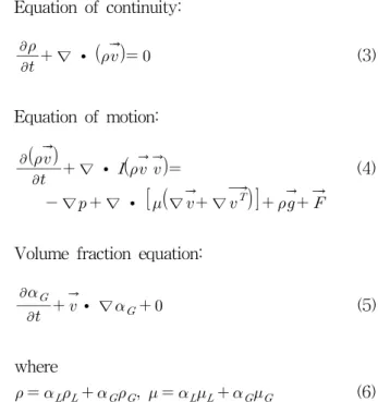
Equation of continuity:



 ∇ ∙





Equation of motion:









 ∇ ∙ 





 ∇  ∇ ∙





^



Volume fraction equation:



_

 ∙ ∇_  (5)

where

  __ __   __ __ (6) The flow is treated as incompressible since the pressure drop along the reactor is small.

Compared to single phase flow simulations, the VOF method accomplishes interface tracking by solving additional continuity-like equation(s) for the volume fraction (n − 1 equations with n as the number of phases)¹⁵⁾. For gas–liquid two phase flows, the volume fraction of gas αG is obtained by numerically solving Eq. (5), and the volume fraction of liquid αL is simply computed from 1 − αG. However, the implementation of the VOF model is numerically challenging. First, both the density ρ and viscosity υ in Eqs. (3) and (4) are mixture properties, which vary within the flow domain and are computed by the volume fraction weighted average in Eq. (6). Second, the interface needs to be constructed based on the computed value of the volume fraction with the application of interpolation schemes for the identification of the interface. Third, surface tension along the interface between each pair of phases, and wall adhesion between the phases and the walls become very important for some cases, especially when the gravitational effect is negligible.

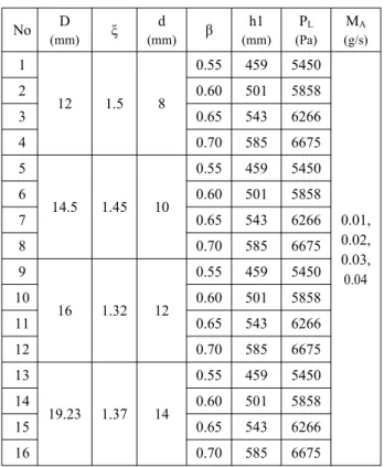
Table 1 Operating conditions for the simulations of water-air flow (T=298K, P=101,325 Pa)

No D

(mm) ξ d

(mm) β h1

(mm) P

(Pa) M

(g/s) 1

12 1.5 8

0.55 459 5450

0.01, 0.02, 0.03, 0.04

2 0.60 501 5858

3 0.65 543 6266

4 0.70 585 6675

5

14.5 1.45 10

0.55 459 5450

6 0.60 501 5858

7 0.65 543 6266

8 0.70 585 6675

9

16 1.32 12

0.55 459 5450

10 0.60 501 5858

11 0.65 543 6266

12 0.70 585 6675

13

19.23 1.37 14

0.55 459 5450

14 0.60 501 5858

15 0.65 543 6266

16 0.70 585 6675

3.2 Numerical approach

The flow inside the micro channel is essentially laminar. As two different fluid met. air bubble and water respectively so surface tension arises as a result of attractive force between molecules in a fluid. and also the adhesion force was taken into account in this paper. In FLUENT, the surface tension model is the continuum surface force (CSF) model proposed by Brackbill et al¹⁷⁾. With this model, the addition of surface tension to the VOF calculation results in a source term in the momentum Eq. (6)¹²⁾. In the case of wall adhesion, a contact angle needs to be specified. Rather than impose the boundary condition at the wall itself, the contact angle that the fluid is assumed to make with the wall is used to adjust the surface normal in cells near the wall. This so-called dynamic boundary condition results in the adjustment of the curvature of the surface near the wall, and this curvature is then used to adjust the body force term in the surface tension calculation¹²⁾. For gas–liquid two phase flows, the source term in Eq. (4) that arises from surface tension can be computed from the following:

  





_∇_

(7)

where κG is the curvature computed from the divergence of the unit surface normal, and σ is the surface tension.

3.3 Comparison of experimental data with numerical predictions

Surface tension of 0.072 N/m, a gas mass rate of 0.01 g/s, 0.02 g/s, 0.03g/s, 0.04 g/s, 0.05 g/s, 0.06 g/s and 0.07 g/s; and wall contact angle of liquid of 60°. The variation of fluid viscosity, surface tension and wall adhesion is also carried out for slug flow development in curved tubes. It is observed that the viscosity, surface tension and wall surface adhesion moderately impact the slug development. The present study will provide insight into the hydrodynamics in curved tubes and will help in further prediction of heat and mass transfer in such devices.

3.4 Simulations

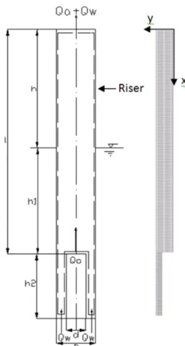
3.4.1. Tube geometry and operating conditions The simulations are carried out in a vertical tube with four different internal diameters D (D=12.00, 14.50, 16.00, 19.23 mm) and this length (L=933m) is like the experiment in the reference¹⁸⁾. Air supply copper tubes with the appropriate injection valves were located coaxially inside the corresponding pump tubes for a length h2=98 mm (suction pipe). The remainder of the tube, have standard length (l=L-h2) is the riser or discharge pipe. The 2D computational domain was divided into 10,000~20,000 rectangle cells. The operation parameters are shown in Table 1 and pointed out in Fig. 2. Near the tube wall, three layers of cells are positioned to assure a correct simulation of the phenomena taking place near the wall. For all simulations, a no-slip condition is imposed at the tube wall. The influence of the gravitational force on the flow has been taken into account. At the inlet of the tube, uniform profiles for all the variables have been employed. A pressure outlet boundary is imposed to avoid difficulties with

backflow at the outlet of the tube.

3.4.2 Solution strategy

Because of the dynamic behavior of the two-phase flow, a transient simulation with a time step of 0.001 s is performed. The calculations are performed by combination of the PISO algorithm¹⁹⁾ for pressure–velocity coupling and a second order upwind calculation scheme²⁰⁾ for the determination of momentum and volume fraction.

3.4.3. Simulation of water–air flow

Fig. 2 Model of air-lift pump

Table 2 Physical properties of water and air (T=298K, P=101,325Pa)

ρ(kg/m3) μ (Pa s) σ (N/m)

Water 998.2

0.001 0.07

Air 1.225

The first part of the simulation work involves 2D, axissymmetry-simulations of the two-phase flow patterns for water and air. For the water–air two-phase system, seven simulation cases under atmospheric pressure and at room temperature have been performed, each one chosen in the center of an operating area representing a different flow regime according to the Baker chart. The

superficial mass velocities of water and air, determined from the Baker chart, are set as inlet conditions for the calculation. The operating conditions are given in Table 1 and pointed out in Fig. 2. Both water and air enter the horizontal tube perpendicular to its inlet plane. They have an inlet temperature of 298 K. The fluid pressure at the tube inlet is set to 101,325 Pa. The physical properties of water and air can be found in Table 2.

4. Result and analysis

Fig. 3 showed the phase profiles in riser from 16.766s to 17.385s in the same air lift pump for D=12.00 mm, submergence ratio of 0.60 and air supply equal to 0.04g/s. The riser length is 0.835m.

During the air phase moving up, from time T1 to time T7, (T1=16.821s, T2=16.857s, T3=16.884s, T4=16.923s, T5=16.955s, T6=16.974s, T7=17.009s,) bubbles merge and split to form a slug shape under the effect of surface tension, gravity, buoyancy, inertia and wall shear force. Maximum slug length is around 10d. Behind the slug bubble always a bubbly tail is formed.

Fig. 4 showed the mass flow rate of water at the outlet of an air lift with a diameter of 12mm, and air supply of 0.04g/s under a submergence rate of 0.6. Mass flow rate is vibrated from 0 to 60 g/s every 0.06s as the air phase shifted to water phase at the outlet boundary. This phenomena is also be examined Fig. 3, every four adjacent phase distribute bars performed one slug flowing out.

The characteristics for riser (D=12mm) and ξ

=1.5. as shown in Fig.5 demonstrate that simulation results, the mass flow rates of air and water, correlate well with the experimental results, Therefore keeping in view this results it is predicted that, this CFD modeling is successful to get the pumping ability of small scale airlift pump.

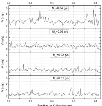
Fig.6 describes the velocity magnitude on X-axis in tube D=12 mm and β=0.60 with different air supply, 0.01 g/s, 0.02 g/s and 0.03 g/s at time

17s. The mean values of velocity are 0.32 m/s, 0.45 m/s, 0.56 m/s 0.83 m/s correspondingly.

Fig. 3 Phase profiles in the riser from 16.766s to 17.385s for D=12mm, β=0.60, MA=0.04 g/s (red-gas slug, blue-liquid slug)

Fig. 4 Mass flow rate of water for D=12 mm, β

=0.60, Ma=0.04 g/s

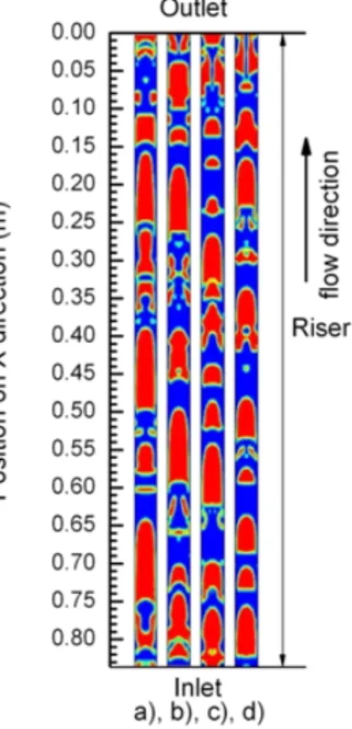
This figure indicated that velocity magnitude increased during increasing the air supply. From figure 6 the curve has been compared. it can be found that the curve with air input equal to 0.04 g/s has the bigger fluctuation than the other curve. Investigated this phenomena together with

Fig. 7, the slug size increase when the air supply increase, from 2d with 0.01 g/s air input and 4d with 0.04 g/s air input. Big size slugs endure bigger buoyancy and have bigger velocity, this make the extended velocity ranged in the flow zone.

Fig. 5 Relationship between volumetric flow rate of water discharge and air supplied for D=12.00mm

Fig. 6 Relationship between velocity magnitude on X-axis and air supply for D=12mm, β=0.60 at 17s

In order to know the trend of changing slug flow, the simulation with air input 0.05 g/s was also carried out continuing the changing air. Since the fraction of air in the flow zone is increased,

bigger slugs will occur. Slugs are getting easier to merge and the slug flow will transit to churn flow.

Fig. 7 Phase distribution in the riser with D=12 mm and β=0.60 at 17s, (a: MA=0.04 g/s; b:

MA=0.03 g/s; c: MA=0.02 g/s; d: MA=0.01 g/s)

5. Conclusion

In this study, A specification and efficiency of the pump was showed up as the mass overcast ratio of the air, the function about the road of the submergence ratio and the length of pipe. The CFD simulation had a similar to the result of an experiment within 10% of dispersion and clarified the gas-liquid flow patterns of two phase in a air lift pump. Especially, the submergence ratio  under 0.5 had more accurate in simulation. When the higher quantity air flow in the tube showed a more fluctuation velocity and had a more unstable with vertical uprising position.

Acknowledgments

This research was financially supported by the Technology Innovation Project of Small and Medium Business Administration, and the National

Research Foundation of Korea Grant funded by the Korean Government (NRF-2010-013-D00007) and 2010 year research professor fund of Gyeongsang National University, Korea.

Reference

1. A. E. Bergeles, 1949. Flow of gas–liquid mixture. Chem. Eng., pp. 104-106.

2. A. H. Stenning, Martin, C.B., 1968. An analytical and experimental study of air lift pump performance. J. Eng. Power, Trans.

ASME Vol. 90, pp. 106-110.

3. B. Storch, 1975. Extraction of sludges by pneumatic pumping. In: Second Symposium on Jet Pumps and Ejectors and Gas Lift Techniques, Churchill College, Cambridge, England, G4, pp. 51-60.

4. Y. Taitel, D. Bornea, A.E. Dukler, 1980.

Modeling flow pattern transition for steady upward gas–liquid flow in vertical tubes.

AICHEJ Vol. 26, pp. 345-354.

5. Hatakeyama, Takahashi, Saito, 1999. A numerical simulation of unsteady flow in an air lift pump. Journal of the Mining and Materials Processing Institute of Japan(Shigen-to-Sozai) Vol. 115, pp. 958-964

6. K. Pougatch, M. Salcudean, 2008. Numerical modeling of deep sea air-lift. International Journal of Ocean Engineering Vol. 35, pp.

1173-1182.

7. Dongying Qian, Adeniyi Lawal, 2006.

Numerical study on gas and liquid slugs for Taylor flow in a T-junction microchannel.

International Journal of Chemical Engineering Science Vol. 61, pp. 7609-7625.

8. E.T. Tudose, M. Kawaji, 1999. Experimental investigation of Taylor bubble acceleration mechanism in slug flow. Chemical Engineering Science Vol. 54, pp. 5761-5775.

9. Donghong Zheng, Xiao He, Defu Che, 2007.

CFD simulations of hydrodynamic characteristics in a gas-liquid vertical upward slug flow. International Journal of Heat and

Mass Transfer Vol. 50, pp. 4151-4165.

10. G.F. Hewitt, D.N. Roberts, 1969, Studies of two-phase flow patterns by simultaneous X-ray and flash photography, UKAEA Report AERE-M2159.

11. V.C. Samaras, D.P. Margaris, 2005. Two-phase flow regime maps for air-lift pump vertical up ward gas-liquid flow. International Journal of Multiphase Flow Vol. 31, pp. 757-766.

12. FLUENT 6.1 documentation, 2003. Fluent Incorporated, Lebanon, New Hampshire.

13. FLUENT application briefs, 2002a-2002d.

Fluent Incorporated, Lebanon, New Hampshire.

14. T., Cui, Z.F., 2006a. CFD modelling of slug flow in vertical tubes. Chemical Engineering Science Vol. 61, 676-687

15. C.W. Hirt, B.D. Nichols, 1981. Volume of fluid (VOF) method for the dynamics of free boundaries. Journal of Computational Physics Vol. 39, pp. 201-225.

16. M.T. Kreutzer, Du, P., Heiszwolf, J.J., F.

Kapteijn, J.A. Moulijn, 2001. Mass transfer characteristics of three-phase monolith reactors. Chemical Engineering Science Vol. 56, pp. 6015-6023.

17. J.U. Brackbill, D.B. Kothe, C. Zemach, 1992. A continuum method for modeling surface tension. Journal of Computational Physics Vol.

100, pp. 335-354.

18. D.A. Kouremenos, J. Staicos, 1985. Performance of a small air-lift pump. International Journal of Heat & Fluid Flow Vol. 6, pp. 217-222 19. R.I. Issa, 1986. Solution of the implicitly

discretized fluid flow equations by operator splitting, J. Comput. Phys. Vol. 62 pp. 40-65.

20. H.K. Versteeg, W. Malalasekera,1995. An Introduction to Computational Fluid Dynamics, the Finite Volume Method, Longman Scientific and Technical, Harlow, Essex, UK, 1995.

21. T. Taha, Z.F. Cui, 2004. Hydrodynamics of slug flow inside capillaries. Chemical Engineering Science Vol. 59, pp. 1181-1190.