1. Introduction1)
With the quantitative growth in water supply pipes in Korea, pipes made of various kinds of materials have been introduced. However, non-systematic repair/maintenance management on networked pipes has led to shorter lifespans than in advanced foreign countries. Furthermore, negative side-effects have arisen
Received 24 November 2015, revised 8 January 2016, accepted 11 March 2016
*Corresponding author: Jayong Koo (E-mail: [email protected])
such as rust due to weak durability and functionality in pipes, in addition to economic loss caused by water leakage. Therefore, the conditions of water mains must be evaluated for sustainable management targeted at more stable and safer water distribution.
Specially, as deterioration and pipe failure in such large-scale water mains pose great potential risk in the case of water leakage, the development of preventive countermeasures would be beneficial, rather than post-accident repair, for example, by putting into action plans to replace deteriorated pipes.
Deterioration Prediction Model of Water Pipes Using Fuzzy Techniques
퍼지기법을 이용한 상수관로의 노후도예측 모델 연구
Taeho Choi1・Min-ah Choi2・Hyundong Lee3・Jayong Koo4*
최태호1・최민아2・이현동3・구자용4
1,2K-water Research Institute, Korea Water Resources Corporation, 125, Yuseong-daero 1689 beong-gil, Yuseong-gu, Daejeon 34045, Republic of Korea
3Environmental Engineering Research Division, Korea Institute of Construction Technology(KICT) and Department of Construction and Environment Engineering, University of Science and Technology(UST), Goyangdae-ro 289, Ilsanseo-gu, Goyang-si, Gyeonggi-do, 10223, Republic of Korea
4(Corresponding author)Department of Environmental Engineering, University of Seoul, Seoulsiripdae-ro 163, Dongdaemun-gu, Seoul, 02504, Republic of Korea
1,2K-water연구원, 3한국건설기술연구원(KICT), 과학기술연합대학원대학교(UST), 4서울시립대학교 환경공학과
ABSTRACT
Pipe Deterioration Prediction (PDP) and Pipe Failure Risk Prediction (PFRP) models were developed in an attempt to predict the deterioration and failure risk in water mains using fuzzy technique and the markov process. These two models were used to determine the priority in repair and replacement, by predicting the deterioration degree, deterioration rate, failure possibility and remaining life in a study sample comprising 32 water mains. From an analysis approach based on conservative risk with a medium policy risk, the remaining life for 30 of the 32 water mains was less than 5 years for 2 mains (7%), 5-10 years for 8 (27%), 10-15 years for 7 (23%), 15-20 years for 5 (17%), 20-25 years for 5 (17%), and 25 years or more for 2 (7%).
Key words: Fuzzy, Remaining life, Risk analysis, Water pipe deterioration prediction model 주제어: 퍼지, 잔존수명, 리스크 분석, 노후도예측 모델
The factors of considering the prediction of the deterioration of water pipe can be divided with three types such as the physical factor, environmental factor, operational factor (Al-Barqawi et al., 2006). There are the pipe material, pipe, wall thickness, pipe age, pipe diameter, type of connection, pipe lining, the form of lining materials, dissimilar metals as the physical factor.
As the environmental factor, there are the types of soil, ground-water, climate, type of backfill, stray current, seismic activity etc. There is the water pressure in the pipe, the water pressure, leakage, water quality, velocity, maintenance activities as the operational factors. Those factors cannot be easily measured or quantified. The prediction of deterioration of water pipe by examining the relations between the factors is more difficult task.
Before the prediction of the deterioration of water pipe, the most common and typical concept about the pipeline life is the “Bathtub Curve” about the pipeline life cycle. The Bathtub Curve means the early burst and the frequency of accidents due to the high failure probability by the initial problems such as the design errors, materials, operating, and the low failure probability is continuously maintained by the stabilization of pipe, but when the years of pipe laying progress increase, in other words, the increase of failure probability due to the end of the life of pipeline, as a result, it shows the direction of increase of the frequency of accidents of pipeline. The management of preventive maintenance before the accident due to the deterioration of the water pipe can extend the life of pipeline (Kleiner et al., 2001).
The methods of prediction of deterioration of water pipe can be divided with two types. First, there is method of using the physical model, second, there is method of using the statistical model. The method of using the physical model is to examine the directness pipe status (presence of scale, degree of corrosion et al.,), the scientific basis has the strong point of securely and widely available, but there is limit of the available data and it takes the data research costs. On the other hand, there are the method of supposing the exponential
function or the linear function with correlation and the method of supposing the already established model such as the regression analysis model, markov process model, Poissons model, cohort living model as the methods of using the statistical model, and it has the strong point to collect the data with the low cost and to be used variously but it has the weak point as the unclear scientific basis.
As the method of using the physical model for the prediction of deterioration of water pipe, there are various study cases such as the deterioration prediction of the steel pipe by Pandey (1998), PVC pipe deterioration prediction by Davis et al.,(2007), and the cast-iron pipe deterioration prediction by Moglia et al.,(2008). And there are the various cases such as the exponential function by Walski(1987), the linear function by Jacob and Karney(1994), markovian process by Kleiner(2001), cohort model by Kropp and Baur(2005), fuzzy technique and markov process by Kleiner(2006), the logistic regression analysis by Park (2008), the random fuzzy technique by Lim(2010), and the artificial neural network by Lee(2010) in the models of using the statistical method.
Especially, the case of studies by Kleiner(2006) case of studies suggested the deterioration prediction model of the water supply pipeline by using the fuzzy technique and markov process, so the subjective and vague deterioration related indicators of water pipe and the objective and quantitative deterioration state can be shown by using the fuzzy technique, and the deterioration transition of the water pipe can be predicted by using markovian process, so in this regard, it is judged as the most effective deterioration prediction model.
But although the various water pipe deterioration prediction method theories, it is difficult to develop the reliable water pipe deterioration prediction model due to the lack of data and inaccuracies of data in Korea.
Therefore, this study aims to develop the water pipe deterioration prediction model using the fuzzy technique and markov process by Kleiner(2006) and to examine its applicability.
2. Methods
2.1 Procedure
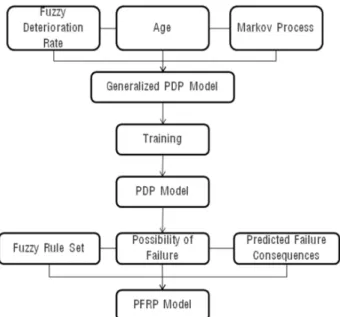
Based on Kleiner (2006)’s development of a reliable decision-making tool for the repair and replacement of deteriorated pipes based on fuzzy technique and the markov process, the present study used the PDP and Pipe Failure Risk Prediction (PFRP) models via the following three-stage process.
In the first stage, the degree of deterioration was determined in 32 large mains of multi-regional waterworks using the indirectness assessment factor, while deterioration factors and their weighting factors were identified.
In the second stage, the PDP model was developed by using fuzzy deterioration to estimate the fuzzificated degree of deterioration in the above first stage, as well as the markov process and pipe ages. The values in deterioration velocity and remaining lifetime of the targeted 32 mains were calculated by controlling the PDP model in such a way as to minimize the summed value of the square of the difference between the predicted value and the actual measured value against fuzzy deterioration.
In the third stage, the PFRP model capable of determining pipe failure risk finalized by using the failure possibility identified by the PDP model and "predicted failure
Fig. 1. Method of PDP and PFRP Modeling.
consequences." The PFRP model was used to determine the degree of failure risk generated as output values through fuzzy algorithm based on such input values as failure possibility and "predicted failure consequences." The model application was successful in determining the in-time period of rehabilitation and readjustment for pipes of water supply system by calibrating the susceptibility of the failure risk to age. Fig. 1 shows the brief procedure followed in developing the PDP and PFRP models.
2.2. Target data
The deterioration of 32 water mains pipelines was assessed using data obtained from the analysis and investigation of multi-regional waterworks and industrial waterworks with respect to facility data, burial environment, pipe state, outer state, inner state, soil corrosivity, microbial characteristics, construction state, management state, historical data, physical strength, chemical composition, and water corrosion. Among these factors, deterioration assessment was carried out with pipelines and assessment indices that showed relatively suitable results and were readily assessable.
The 32 pipelines were largely used for conveying raw water, treated water, or industrial water. The pipe material was CIP, DCIP, SP, or PC, and they were mostly large pipes with diameters ranging from 300mm to 2,200mm.
2.3 Deterioration assessment
The local 'Manual for Diagnosing Water Supply Piping Network' requires such assessment items as indirect evaluation factors, direct evaluation factors, and corrosion-impacting factors to determine more about structural safety. Indirect evaluation factors were mainly adopted owing to easier accessibility and better accuracy to related data, which detailed as pipe material, pipe diameter, inner coating, outer coating, age of use, type of soil, traffic type, connection type, leakage and failure recording, and occurrences of claim-petitioning such as water quality/pressure. The nine aforementioned subfactors were incorporated in the study by excluding the last subfactor of occurrences of claim-petitioning due to statistical insufficiency.
The 9 deterioration assessment indices are shown in Table 1 Here, the state of deterioration assessment indices is divided into diverse grades of 3, 4, 5 or 6. The state of each assessment index was rated on the following 7-point grade scale to ensure consistent evaluation of the states of deterioration assessment indices: Excellent, Good, Adequate, Fair, Poor, Bad, and Failed.
The indirectness assessment items do not necessarily have the same effects on water main deterioration. Therefore, calculating the deterioration of a water main necessitates calculating the weighting values of indirectness assessment items. Since this study does not examine the weighting values of indirectness assessment items that affect the deterioration of water mains, the existing literature (Deteriorated Water Main Assessment and Management Manual, 2002) was cited.
Consequently, the weighting value by indirectness assessment item was determined to be 0.22 for material, 0.11 for diameter,
0.08 for inner coating, 0.02 for outer coating, 0.20 for age, 0.06 for soil, 0.06 for traffic type, 0.02 for connection type, and 0.23 for leakage and failure recording, with the total of the weighting values being 1.
2.4. PDP Modeling
The degree of deterioration was calculated by multiplying the weighting value by the graded subfactor, the result of which was further converted into fuzzy deterioration through fuzzification with 9 membership values. The fuzzy deterioration in case of time t is expressed by Eq. 1 as follows;
(Eq. 1)
where, : Fuzzy deterioration in case of time t : Membership value as to time t and triangular
membership Table 1. Indirectness assessment index and classification scope
Index Classification
scope Value State Index Classification
scope Value State
1.
Material
CIP, GSP PVC, PE SP, PC, PCC
DCIP STS, PFP
1.00 0.75 0.50 0.25 0.00
Bad Poor Fair Adequate
Good
6. Soil
Clay Clay+Gravel, Silt Sand+Gravel, Loam
Sand
1.00 0.50 0.25 0.00
Failed Poor Adequate Excellent
2.
Diameter
<=150mm 150 ~ 350mm 350 ~ 600mm 600 ~ 1000mm 1000~ 2000mm
>2000mm
1.00 0.80 0.60 0.40 0.20 0.00
Bad Poor Fair Adequate
Good Excellent
7.
Traffic type
Highway
>4 lane road 2 lane road
Local road Footway
1.00 0.75 0.50 0.25 0.00
Bad Poor Fair Adequate
Good
3.
Inner coating
No Epoxy Coaltar enamel
Asphalt Cement mortar
1.00 0.75 0.75 0.50 0.00
Bad Poor Fair Adequate
Good
8.
Connectio n method
Sleeve coupling Flange, Socket heat anastomosis Mechanical,Push-on J.
Coating after welding
1.00 1.00 0.50 0.25 0.25
Bad Poor Fair Adequate
Good 4.
Outer coating
No Coaltar enamel
Asphalt
1.00 0.75 0.00
Bad Fair Good
9.
Leakage and failure
recording
>5times/5year-50km 3~5times/5year-50km 1~3times/5year-50km
No
1.00 0.50 0.25 0.00
Failed Poor Adequate Excellent
5.
Age
>25year 20 ~ 25year 15 ~ 20year 10 ~ 15year
<=10year
1.00 0.75 0.50 0.25 0.00
Bad Poor Fair Adequate
Good
In the current state as the water pipe condition the fuzzy deterioration of the pipeline has spread as by the transition matrix using the markov process as the concept which is influenced on the verge stage. If markov process concept is used sequentially by the time sequence after the water pipe is layed, value about whole life of water pipe can be expressed. In other words, markov process is the tool for prediction of value progress through the transition matrix in the conceptual aspect in the future. It can be expressed by Eq. 2 as follows;
⊗ (Eq. 2)
Eq. 2 has two pre-assumptions: firstly, water mains are not capable of improvement without external intervention as expressed by when all . Secondly, pipes suffer relatively slow but continual natural deterioration, thus concluding that triangular membership, , is processed to deterioration, if time is in short for deterioration (Kleiner, 2001). Therefore, Eq. 3 is drawn when is formed as a matrix using the above assumptions.
(Eq. 3)
⋯
where, is the deterioration rate when triangular membership, , in time is transformed to deterioration,
. For example, means the degree of deterioration rate when triangular membership 1(excellent) in time t is transformed to triangular membership 2(good). Likewise, if =0.05, 5% membership value in triangular membership, , is transformed to triangular membership,
when the deterioration of pipes is transformed from time to time . In other words, No. membership value included in spreads No. membership value by , or can be spread as No. membership value, and it means to calculate using markov process concept by the flow of time of the water pipe.
Eq. 3 shows that the fuzzy deterioration in pipes is gradually absorbed to failed triangular membership. In such cases, however, the analysis is too complicated to be non-realistic because the fuzzy deterioration in pipes shall be expressed only through numerous triangular memberships. Therefore, the threshold value, , is introduced to reduce the distribution of triangular membership to 7 grades, subject to the pipe conditions. acts to control the value of membership when triangular membership flows to change to in time , which means the value of membership in triangular membership is restricted unless otherwise exceeded by threshold value in a certain time prior to . To represent this, Eq. 4 is formed by introducing to Eq. 3.
⋯
max ≥ ≤
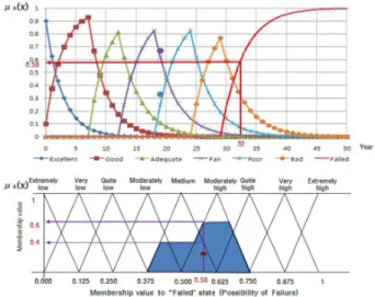
(Eq. 4)Fig. 2 shows the diagram extracted from Eq. 4.
Fig. 2. Deterioration curves with membership thresholds Therefore, when and in Eq. 4 vary in the deterioration prediction model, the shape of the deterioration curve in Fig. 2 is changed. Using this method, PDP modeling was finalized in the pertinent piping network so as to minimize the summed value of the square of the difference between the predicted value and actual measured value.
2.5 PFRP Modeling
The pipe failure risk was estimated through fuzzy algorithm using rule-base by setting as input values the failure possibility (frequency) depending on the age of time elapse in the failed curve of PDP the model, as well as the "predicted failure consequences (damaged magnitude)".
2.5.1 Failure Possibility (Frequency)
The failure possibility as in the PFRP model can be extractable from the "failed" curve by the age of time elapse in the PDP model. For example, when Pipe No. CW-01
Fig. 3. Re-mapping of membership values in the “Failed” state onto the “Possibility of Failure” fuzzy set
is superannuated with an age of 32 years, the resultant failure possibility is 0.58, which can be expressed following fuzzification by the diagram shown in Fig. 3.
2.5.2 Predicted Failure Consequences (Damaged Magnitude)
"The predicted failure consequences" can be determined according to the water supply connection, pipe diameter and use purpose of the pipe. By focusing on the fact that volumetric water flowability is directly dependant on the size of the pipe diameter, this study adopted a subfactor of pipe diameter as the determinants for "predicted failure consequences"; more specifically, by relying on lost water volume in the case of pipe fracture (failure) and the number of households cut off for water supply by using fuzzy technique based on the 9 grades (from extremely low to extremely severe). For example, the "predicted failure consequences"
for the 400mm-pipe can be expressed as shown in Fig. 4
Fig. 4. Fuzzification of predicted failure consequences Table 2. Fuzzy rule-set for failure possibility and consequence relationship
Possibility of Failure
Predicted Failure Consequences Extremely
low
Very low
Quite low
Moderately
low Medium Moderately severe
Quite severe
Very severe
Extremely severe
Extremely low EL EL VL VL QL QL ML ML M
Very low EL VL VL VL QL ML M M MH
Quite low VL VL QL QL ML ML M M MH
Moderately low QL QL QL QL ML M M MH QH
Medium QL ML ML ML M M MH MH QH
Moderately high ML ML ML ML M MH MH QH VH
Quite high ML M M M MH MH QH QH VH
Very high M M M M MH QH VH VH EH
Extremely high M MH MH MH QH VH VH EH EH
EL : Extremely low, VL : Very low, QL : Quite low, ML : Moderately low, M : Medium, MH : Moderately high, QH : Quite high, VH : Very high, EH : Extremely high
showing that membership values are 0.66 for Very-Low triangular membership, 0.33 for Quite-Low triangular membership, and zero for the remaining grades.
2.5.3 Fuzzy Rule-set
To execute the fuzzy algorithm, with the possibility of failure and "the predicted failure consequences" being the input and the failure risk being as the output, rules that control the input and output values of the fuzzy algorithm are necessary.
The fuzzy rule-set consists of the rules that control the input and output values of the fuzzy algorithm, and refers to the failure risk for the possibility of failure and "the predicted failure consequences" at the number of all cases.
This study used a generalized fuzzy rule-set, as shown in Table 2. The proposed fuzzy rule-set, however, is fully modifiable based on empirical grounds. It is deemed that the reliability of the result value will be increased if the fuzzy rule-set is modified and supplemented with optimal values at the stage of utilizing the development result.
3. Results and Discussion
3.1 Deterioration assessment
The deterioration of the 32 pipelines can be determined by applying weighting values of indices to their graded values of indices, as shown in Table 3.
The deterioration of a pipeline has a value between 0 and 1. The nearer to 0 the deterioration, the better the pipeline,
and the nearer to 1 the deterioration, the poorer the pipeline.
Pipeline No. GS-01 showed a deterioration of 0.242, and was the best pipe. Pipeline No. CW-03 showed a deterioration of 0.749, and was the poorest pipe. These data on pipeline deterioration, however, are only relative, not absolute, values for determining the degree of deterioration. The current state of a pipeline cannot be determined only with the deterioration of the pipeline, which is judged to be quite insufficient as grounds for deciding at which time in the future the pipeline should be renewed or replaced. Therefore, it is deemed that the deterioration of pipelines calculated in this section has limitations.
3.2. Fuzzy deterioration assessment
To apply the deterioration of pipelines calculated above to the PDP model, it should be converted to the fuzzy deterioration. The results of converting the deterioration of the 32 pipelines to the fuzzy deterioration are s shown in Table 4.
Just like the deterioration of the 32 pipelines obtained above, pipeline No. GS-01 shows the best fuzzy deterioration, which may be expressed as (0, 0.54, 0.46, 0, 0, 0, 0); and pipeline CW-03 shows the poorest fuzzy deterioration, which may be expressed as (0, 0, 0, 0, 0.5, 0.5, 0).
3.3. Results of the PDP Model
If the PDF model is trained with the fuzzy deterioration of the 32 pipelines, the threshold values of and Table 3. Deterioration rate analysis result of pipes
Pipe ID Deterioration rate Pipe ID Deterioration rate Pipe ID Deterioration rate
CW-01 0.556 GJ-01 0.330 GJ-03 0.421
CW-02 0.408 PH-01 0.571 KG-02 0.407
CW-03 0.749 GM-02 0.420 KG-03 0.415
CW-04 0.731 CJ-01 0.250 US-02 0.392
SD-01 0.472 GJ-02 0.668 NG-05 0.459
GS-01 0.242 NG-04 0.404 NG-06 0.459
GM-01 0.605 US-01 0.512 GM-03 0.313
CW-05 0.477 KG-01 0.447 GJ-04 0.489
NG-01 0.353 YC-01 0.370 GJ-05 0.561
NG-02 0.376 CW-06 0.731 GM-04 0.433
NG-03 0.377 CW-07 0.628
*Bold letters indicate the maximum and minimum values
have values that minimize the sum of squares of deviation for the measured and predicted values.
Under the assumption that fuzzy deterioration at the time of underground laying was (0.9, 0.1, 0, 0, 0, 0, 0), the critical values in each triangular membership were applied
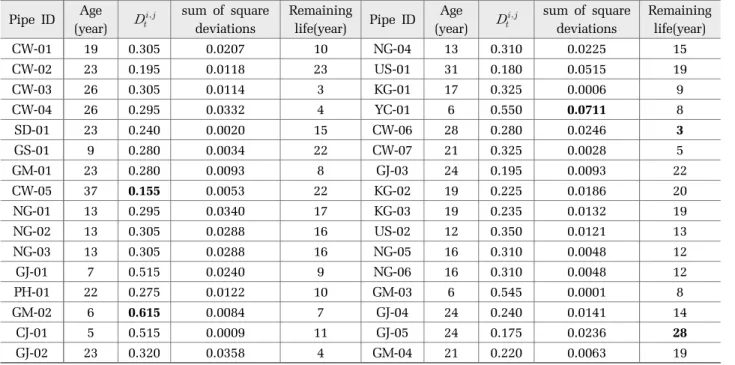
by (- , 0.9, 0.8, 0.8, 0.8, 0.7, -). Similarly, when fuzzy deterioration was computed for all 32 pipe mains, the values, added values of difference square and remaining lifetime could be determined in each pipe main. The results are shown in Table 5.
Table 4. Fuzzy deterioration rate of pipes
Pipe ID Fuzzy deterioration rate Pipe ID Fuzzy deterioration rate CW-01 (0, 0, 0, 0.670, 0.330, 0, 0) NG-04 (0, 0, 0.580, 0.420, 0, 0, 0) CW-02 (0, 0, 0.550, 0.450, 0, 0, 0) US-01 (0, 0, 0, 0.930, 0.070, 0, 0) CW-03 (0, 0, 0, 0, 0.500, 0.500, 0) KG-01 (0, 0, 0.130, 0..870, 0, 0, 0) CW-04 (0, 0, 0, 0, 0.620, 0.380, 0) YC-01 (0, 0, 0.780, 0.220, 0, 0, 0) SD-01 (0, 0, 0.170, 0.830, 0, 0, 0) CW-06 (0, 0, 0, 0, 0.620, 0.380, 0) GS-01 (0, 0.540, 0.460, 0, 0, 0, 0) CW-07 (0, 0, 0, 0.230, 0.770, 0, 0) GM-01 (0, 0, 0, 0.370, 0.630, 0, 0) GJ-03 (0, 0, 0.480, 0.520, 0, 0, 0) CW-05 (0, 0, 0.130, 0..870, 0, 0, 0) KG-02 (0, 0, 0.550, 0.450, 0, 0, 0) NG-01 (0, 0, 0.880, 0.120, 0, 0, 0) KG-03 (0, 0, 0.520, 0.480, 0, 0, 0) NG-02 (0, 0, 0.730, 0.270, 0, 0, 0) US-02 (0, 0, 0.640, 0.360, 0, 0, 0) NG-03 (0, 0, 0.730, 0.270, 0, 0, 0) NG-05 (0, 0, 0.250, 0.750, 0, 0, 0) GJ-01 (0, 0.020, 0.980, 0, 0, 0, 0) NG-06 (0, 0, 0.250, 0.750, 0, 0, 0) PH-01 (0, 0, 0, 0.570, 0.430, 0, 0) GM-03 (0, 0.120, 0.880, 0, 0, 0, 0) GM-02 (0, 0, 0.480, 0.520, 0, 0, 0) GJ-04 (0, 0, 0.070, 0.930, 0, 0, 0) CJ-01 (0, 0.500, 0.500, 0, 0, 0, 0) GJ-05 (0, 0, 0.630, 0.370, 0, 0, 0) GJ-02 (0, 0, 0, 0, 0.990, 0.010, 0) GM-04 (0, 0, 0.400, 0.600, 0, 0, 0)
*Bold letters indicate the maximum and minimum values
Table 5. PDP model training result of pipes Pipe ID Age
(year) sum of square deviations
Remaining
life(year) Pipe ID Age
(year) sum of square deviations
Remaining life(year)
CW-01 19 0.305 0.0207 10 NG-04 13 0.310 0.0225 15
CW-02 23 0.195 0.0118 23 US-01 31 0.180 0.0515 19
CW-03 26 0.305 0.0114 3 KG-01 17 0.325 0.0006 9
CW-04 26 0.295 0.0332 4 YC-01 6 0.550 0.0711 8
SD-01 23 0.240 0.0020 15 CW-06 28 0.280 0.0246 3
GS-01 9 0.280 0.0034 22 CW-07 21 0.325 0.0028 5
GM-01 23 0.280 0.0093 8 GJ-03 24 0.195 0.0093 22
CW-05 37 0.155 0.0053 22 KG-02 19 0.225 0.0186 20
NG-01 13 0.295 0.0340 17 KG-03 19 0.235 0.0132 19
NG-02 13 0.305 0.0288 16 US-02 12 0.350 0.0121 13
NG-03 13 0.305 0.0288 16 NG-05 16 0.310 0.0048 12
GJ-01 7 0.515 0.0240 9 NG-06 16 0.310 0.0048 12
PH-01 22 0.275 0.0122 10 GM-03 6 0.545 0.0001 8
GM-02 6 0.615 0.0084 7 GJ-04 24 0.240 0.0141 14
CJ-01 5 0.515 0.0009 11 GJ-05 24 0.175 0.0236 28
GJ-02 23 0.320 0.0358 4 GM-04 21 0.220 0.0063 19
*Bold letters indicate the maximum and minimum values
Application of the PDP model revealed that GM-02 showed the highest deterioration rate of 0.615, and that CW-05 showed the lowest deterioration rate of 0.155. CW-06 and CW-03 had the shortest remaining life of 3 years, and GJ-05 had the longest remaining life of 28 years. Analysis of the mean deterioration rates by material revealed that CIP had a mean deterioration rate of 0.305, DCIP 0.343, and SP 0.307. In conclusion, combining the results of deterioration rate and remaining life revealed that pipeline Nos. CW-03, CW-04, GJ-02, CW-06, and CW-07 should be given priority for improvement or replacement. Nevertheless, the results from the PDP model need to be applied to the PFRP model in order to predict the deterioration more accurately and logically.
3.4 Results of the PFRP Model
Pipe failure risk was predicted according to the age of pipes by taking full advantage of 'failure possibility', 'predicted failure consequences' and 'rule-set' extracted from the PDP model. Accordingly, the result for CW-01 is shown in Fig.
5, which demonstrates that all other cases are equivalently computable.
The failure risk in the study can be expressed by defuzzified failure risk, conservative failure risk and optimistic failure risk. To strengthen safety in piping, optimistic failure risk may be preferable to conservative failure risk because, even in the case of the same risk, the conservative failure risk has earlier renewal and replacement than the optimistic failure risk.
Fig. 5. PFRP model result of Pipe ID CW-01.
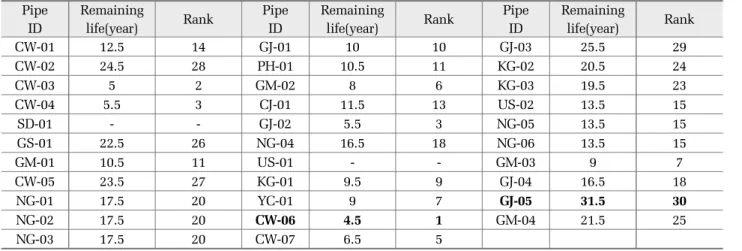
Unlike in the PDP model, the remaining life in the PFRP model can be applied flexibly according to failure risk, conservative failure risk or optimistic failure risk. For example, in the event that the conservative failure risk is determined when the risk caused by policy is set as medium, the results through the PFRP model against all 32 mains are made as shown in Table 6 according to the priority in repair and replacement, i.e., the order of remaining life.
From this analysis with a medium level of policy risk and a conservative failure risk, among the 30 pipelines, excluding 2 whose remaining life could not be obtained, 2 pipelines (7%) had a remaining life of 5 years, 8 (27%) of 5-10 years, 7 (23%) of 10-15 years, 6 (20%) of 15-20 years, 5 (17%) of 20-25 years, and 2 (7%) of more than 25 years.
Table 6. Remaining life at medium and conservative risk levels Pipe
ID
Remaining
life(year) Rank Pipe ID
Remaining
life(year) Rank Pipe ID
Remaining
life(year) Rank
CW-01 12.5 14 GJ-01 10 10 GJ-03 25.5 29
CW-02 24.5 28 PH-01 10.5 11 KG-02 20.5 24
CW-03 5 2 GM-02 8 6 KG-03 19.5 23
CW-04 5.5 3 CJ-01 11.5 13 US-02 13.5 15
SD-01 - - GJ-02 5.5 3 NG-05 13.5 15
GS-01 22.5 26 NG-04 16.5 18 NG-06 13.5 15
GM-01 10.5 11 US-01 - - GM-03 9 7
CW-05 23.5 27 KG-01 9.5 9 GJ-04 16.5 18
NG-01 17.5 20 YC-01 9 7 GJ-05 31.5 30
NG-02 17.5 20 CW-06 4.5 1 GM-04 21.5 25
NG-03 17.5 20 CW-07 6.5 5
*Bold letters indicate the maximum and minimum values
4. Conclusion
Both PDP and PFRP models were developed in an attempt to predict the deterioration and failure risk in water mains using fuzzy technique and the markov process. These two models were used to determine the priority in repair and replacement, by predicting the deterioration degree, deterioration rate, failure possibility and remaining life of 32 water mains.
Although the PDP model was found to be effective in determining the approximate timing for rehabilitation and replacement, using the model for prediction was difficult when the deterioration was already in process. On the contrary, the PFRP model could be applied flexibly, regardless of ongoing deterioration; hence, this model is likely to be the fittest for determining the timing of repair/replacement when the related data is accumulated. From an analysis approach based on conservative risk with a medium policy risk, the remaining life for 30 of the 32 water mains was as follows:
2 mains (7%) showed a remaining life of less than 5 years, 8 (27%) of 5-10 years, 7 (23%) of 10-15 years, 6 (20%) of 15-20 years, 5 (17%) of 20-25 years, and 2 (7%) of 25 years or more.
Thus, this study calculated the deterioration prediction and remaining life based on only 32 pipeline as subjects.
But it is judged that more selections of the analysis case on the water pipe and the verification water pipe of same type should be needed for the reliability improvement of PDP model and PFRP model. Especially, the data which was used for PDP model and PFRP model in this study is the indirectness assessment factor about the pipe deterioration, so the factor which can be changed with time is only the pipe age factor among the indirectness assessment factors. In this case, the measurement of the deterioration by the specific time interval about the same water pipe cannot classify the difference between the actual measurement value and the prediction value by the model definitely. But if the directness assessment factors such as the physical strength of capsule and chemical composition, etc. which is changed with the time are applied to PDP model and PFRP model which was suggested in this study, it is judged that will be used enough as the validation data for the reliability
of this model.
In other words, it can be used enough for the water pipe deterioration of PDP model and PFRP model using the indirectness assessment factor and for the remaining life prediction, and it is judged that will be used more effectively for determining the renewal and replacement priorities and time of aging water pipe by drawing reliable result rather than the case that the directness assessment factor about the water pipe deterioration assessment is managed and used continually in Korea.
References
Al Barqawi, H. and Zayed, T., 2006, Condition rating model for underground infrastructure sustainable water mains, J. Perform. Constr. Facil, 20(2), pp.126-135
Kleiner, Y. and Rajani, B., 2001a. Comprehensive review of structural deterioration of water mains: Physically based models, Urban Water, 3(3), pp.151-164
Kleiner, Y. and Rajani, B., 2001b. Comprehensive review of structural deterioration of water mains: Statistical models, Urban Water, 3(3), pp.131-150
Pandey, M.D., 1998. Probabilistic models for condition assessment of oil and gas pipelines, NDT & E International, 31(5), pp.349-358
Davis, P., Burn, S., Moglia, M. and Gould, S., 2007. A physical probabilistic model to predict failure rates in buried PVC pipelines, Reliability Engineering & System Safety, 92(9), pp.1258-1266
Moglia, M., Davis, P. and Burn, S., 2008. Strong exploration of a cast iron pipe failure model, Reliability Engineering
& System Safety, 93(6), pp.885-896
Walski, T. M., 1987. Replacement rules for water mains, Journal of the American Water Works Association, 79(11), pp.33-37 Jacobs, P. and Karney, B., 1994. GIS development with
application to cast iron main breakage rate, Proc., 2nd Int. Conf. on Water Pipeline Systems, BHR Group Ltd., Edinburgh, Scotland.
Kleiner, Y., 2001. Scheduling inspection and renewal of large infrastructure assets, Journal of infrastructure Systems, 7(4), pp.136-14
Kropp, I. and Baur, R., 2005. Integrated failure forecasting model for the strategic rehabilitation planning process, Water Science & Technology : Water Supply, 5(2), pp.1-8 Kleiner, Y., Rajani, B. B. and Sadiq, R., 2006. Modeling the
deterioration and managing failure risk of buried critical infrastructure, National Research Council Canada, pp.294-306
Park, S. B., 2008. Development of a probability model for water main burst risks using the leakage type analysis methods, University of Seoul
Lim, K. Y., 2011. Assessment of the priorities for rehabilitation
of water pipes using the fuzzy techniques, Pusan National University
Lee, M. R., 2010. A Study on deterioration evaluation model of water main using integrated PCA and ANN, University of Seoul
Yoon, J. H. et al., 2002. Deteriorated water main assessment and management manual, Ministry of Environment