A study on the classification of households in Rwanda based on factor scores

A study on the classification of households in Rwanda based on factor scores

Pacifique Nizeyimana ¹ · Kee-Won Lee ² · Songyong Sim ³

123 Department of Statistics, Hallym University

Received 17 February 2018, revised 13 March 2018, accepted 14 March 2018

Abstract

Many researchers have focused on grouping or classifying households into different categories based on either income/consumption or household assets. However, these practices may lead to an inadequate classification due to Rwanda’s unique family struc- ture. In Rwanda, households are classified into six socio-economic classes known as

‘Ubudehe categories’. This classification is based on subjective perceptions of people.

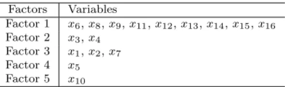
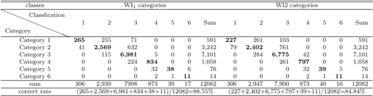
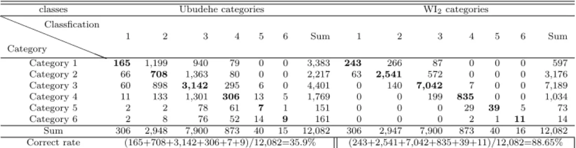
In this study, we propose to use household assets as well as income/consumption to classify Rwandan households into different socio-economic categories. These approaches are summated Likert scale method and factor score method. When these two meth- ods are compared by a discriminant analysis, the factor score method brings out more reliable results than Likert method.

Keywords: Factor score, household assets, summated Likert scale, Ubudehe categories, wealth index.

1. Introduction

As a developing country, Rwanda has a vision of fighting against poverty and improving the welfare of its population. One way the Rwandan government has sought to improve the welfare of its people is by classifying households into categories based on individual living standards and economy. These categories are commonly known as “Ubudehe categories”.

In 2001, the government reintroduced Ubudehe as a process whereby people from the same cell come together to evaluate their current living situations, and decide on solutions to improving development. In this process, the heads of households from the same cell come together and classify themselves into six different socio-economic categories, ranging from the poorest households (Category 1) to the richest households (Category 6). The main goals of this practice of Ubudehe are as follows:

1. To fight against poverty.

1

Graduate student, Department of Statistics, Hallym University, Chuncheon 24252, South Korea.

2

Professor, Department of Statistics, Hallym University, Chuncheon 24252, South Korea.

3

Corresponding author: Professor, Department of Statistics, Hallym University, Chuncheon 24252, Ko-

rea. E-mail: [email protected]

2. To identify eligible beneficiaires for pro-poor programs, financial aids in education, direct support, social protection programs, public work distribution, financial services, health insurance, and other programs with the aim of poverty reduction and general development.

This system of Ubudehe categories was implemented in all sectors of the country. Since then, the government has used these categories to decide who are eligible for special aid or help in order to increase development within a category. However, it is important to note that:

1. The classification is established based on individual perceptions of poverty and wealth within a cell.

2. The Rwandan government typically has only provided aid to those in the first two categories (Category 1 and Category 2), many types of aid are provided (Devereux, 2012).

This method of classification of socio-economic categories might probably has some flaws due to biased perceptions, and emotions, or conflicts within the community. Since the government started using this classification, people have been claiming about their clategories, many student dropped the school as the consequences of this classification. Transparency Rwanda announced that Ubudehe categories does not represent the economic status.

We classify households into different categories using statistical methods such as summated Likert method and factor score method. Classifications based on socio-ecomic status or poverty level are studied. These include Citro (1995), Kaufman and Rousseeuw (1990) and Falkingham and Namazie (2002). For the calculations, we use SPSS (IBM Corp., 2013) and R (Cabacoff, 2015; R Core Team, 2017).

We used the data from National Institute of Statistics of Rwanda survey known as (EICV4). Details of the data are given in Section 2. In Section 3, we propose statistical scoring methods above mentioned and finally, we compare those methods with Ubudehe categories in Section 4.

2. Data

2.1. Source of data and data preparation

The data that we will use in this study is from Integrated Household Living Condition Survey known in French as Enquete Integrale sur les Conditions de Vie (EICV4), which was conducted in 2013/14. The sample size is 14,419 households, taken randomly from all districts of Rwanda. The EICV4 conducted in 2013/14 is the follow-up to the 2000/01, 2005/06 and 2010/11 surveys. Each survey provides information on monetary poverty measured in consumption expenditure terms. It also provides some information which indicate the change of living conditions of households in Rwanda.

In total 14,419 households from all the district of the country participated in the survey

EICV4, 2,337 households, which is equivalent to 16.2%, were not found on the list of Ubudehe

classification (not classified for unknown reasons). Therefore, they were considered in this

study as missing and they were excluded in this study. Finally 12,082 households were eligible

for inclusion in this study. The following variables are used in our analysis: region, type of

dwelling, house owner, poverty level, Ubudehe category, consumption expenditure, type of

residency, current dwelling value, water source, light source, amount paid for electricity in the last 4 weeks, primary source of cooking fuel, type of toilet, roofing materials, main construction materials, floor materials, floor area. Many of these variables are categorical variables, not ordered. For this reason, the first step in this analysis is preparing data by weighting indicator variables in an ascending way, where the cheapest asset will be assigned the lowest value, and most expensive asset will be assigned the highest value.

For example, for the variable main construction material we assign “1” for sheeting, “11”

for tree trunk with mud , “7” for stones and “9” for cement bricks.

In the case of region variable, living expenses are not the same across regions. Therefore, we assign a lower value where the living expense are lower, and a higher value where living expenses are higher. In the region variable, we assign “1” for the rural north, in which life is the most inexpensive in the country, while we assign 6 for Kigali city, the capital, where life is most expensive in Rwanda. In the case that it is neither assets nor location we consider affordability. The assets that are affordable by the rich are assigned a high score. Otherwise, we assign a low score.

All the variables are on a different scale, that is why we standardized all categorical variables.

2.2. Relationship between Ubudehe categories and other variables 2.2.1. Poverty, quantile and Ubudehe classification

We compare the Ubudehe classification and household consumption expenditure. The household expenditure is obtained from the same data set of EICV4. The data set of EICV4 already has a variable called ‘poverty’ and it classifies households into one of three categories:

very poor, poor, or not poor. There are many methods to measure poverty including Citro and Michael (1995). Based on main indicators report of integrated household living condi- tions survey (National instute of statistics of Rwanda, 2015), the variable ‘poverty’ is based on household consumption expenditure, which classifies the households that consume less than RWF (Rwandan Francs) 105,064 per year as very poor, the households that consume between RWF 105,064 and RWF 159,375 (exclusively) per year as poor, and the households that consume more than or equal to RWF 159,375 per year as not poor. This bracket RWF 105,064 and RWF 159,375 are set by the national institute of statistics of Rwanda (NISR).

Note that RWF stands for Rwandan Francs, which is the official monetary unit in Rwanda.

Both figures provide visual comparisons of Ubudehe categories with both poverty and quantiles. We can see in Figure 2.1a, there seems to be some inconsistency in Ubedehe classification and the variable poverty.

For example, there are some households in Ubudehe category 1 that are actually classified as ‘not poor’. This means these housholds receive the most governmental aids while they are

‘not poor’. This also occurs in the households of Ubedehe category 2 that are ‘not poor’.

From Figure 2.1a, we can also see that the majority of households classified as ‘very poor’

are included in Category 3, while they should be in Category 1 or Category 2 if Ubudehe and

poverty are truly consistent. Looking at the category 1 in Figure 2.1b, we observe households

which belongs actually to Q 3 , Q 4 and Q 5 the richest. These households should belongs to

Q ₁ or Q ₂ if there is consistency. We can conclude that Ubudehe categories do not correlate

well with poverty and consumption.

(a) Ubudehe and Poverty (b) Ubudehe and Quantile Figure 2.1 Ubudehe and poverty, Ubudehe and quantile

3. Methods

3.1. Likert scale method

For scoring or measuring an abstract thing, Likert scale has been used (Likert, 1932; Kim et al., 2016). We use Likert scale for scoring household wealth.

3.1.1. Wealth index 1

Let x _ij be the observed value of the j-th household of i-th variable. Since each variable has different mean and variance, we use a standardized variable

Z ij = x _ij − ¯ x _i s i

, (3.1)

where ¯ x i and s i are the mean and standard deviation of x ij ’s.

We first tried to use a wealth index as follows (we omit j subscript hereafter for briefness):

WI 1 = Z 1 + Z 2 + ... + Z 17 . (3.2) However, we could not use the variable ‘amount paid for electricity’ because more than 70%

of observation is missing. Therefore, we finally can add up the remaining 16 variables to make a wealth index for each household as

WI 1 =

16

X

i=1

Z i . (3.3)

3.2. Factor analysis

Lee and Sim (2016) proposed to use factor scores for scoring. We apply their scoring.

See also Kwak and Rhee (2016). To get the score for the households, we perform a factor analysis with varimax rotation method to obtain orthogonal factors. We find 5 factors that have eigenvalues larger than one. The variables that belong to each factor are summarized in Table 3.1.

Table 3.1 Factors and their corresponding variables Factors Variables

Factor 1 x

, x

, x

, x

, x

, x

, x

, x

, x

Factor 2 x

, x

Factor 3 x

, x

, x

Factor 4 x

Factor 5 x

3.2.1. Weighting factors

We apply a simlified version of Lee and Sim (2016)’s scoring of each household. Denote the eigenvalues obtained by the factor analysis as λ ₁ > λ ₂ > · · · > λ _m > 1 and

T i =

√ λ 1 F ˆ 1 + √

λ 2 F ˆ 2 + ... + √ λ m F ˆ m

q P m j=1 λ j

, (3.4)

where

F ˆ k = P a

j=a

+1 L j Z ij

s _k , (3.5)

where s ² _k is the variance of P a

j=a

+1 L _j Z _ij . We consider the wealth of every household using factors

WI 2 = a 1 F ˆ 1 + a 2 F ˆ 2 + a 3 F ˆ 3 + a 4 F ˆ 4 + a 5 F ˆ 5 . (3.6) By a factor analysis we have ˆ F 1 = Z 6 + Z 8 + X 9 + Z 11 + Z 12 + Z 13 , ˆ F 2 = Z 3 + Z 4 , F ˆ 3 = Z 1 + Z 2 + Z 7 , ˆ F 4 = Z 5 , and ˆ F 5 = Z 10 so that the wealth index becomes

WI 2 = a 1 (Z 6 + Z 8 + Z 9 + Z 11 + Z 12 + Z 13 ) + a 2 (Z 3 + Z 4 )

+a 3 (Z 1 + Z 2 + Z 7 ) + a 4 Z 5 + a 5 Z 10 , (3.7) where

a _i =

√ λ k

q P k j=1 λ _j

. (3.8)

From the data, we calculated a ₁ , a ₂ , a ₃ , a ₄ and a ₅ . The calculation gives a ₁ = √ 3.904, a ₂ = √

1.930,a ₃ = √

1.153, a ₄ = √

1.089 and a ₅ = √

1.001, so that the wealth index is

WI 2 = √

3.904(Z 6 + Z 8 + Z 9 + Z 11 + Z 12 + Z 13 ) + √

1.930(Z 3 + Z 4 ) + √

1.153(Z 1 + Z 2 + Z 7 ) + √

1.089Z 5 + √

1.001Z 10 . (3.9)

3.3. Comparison between WI 1 categories and WI 2 categories

The classification problem on hand does not have a reference to be compared. Therefore, we will perform discriminant analysis to compare two scoring methods: one is based on WI ₁ , and the other is WI ₂ (Kim and Hong, 2017).

Since we use discrimant analysis to make comparisons of different classifications, the first step is to find the best reference among WI 1 categories and WI 2 categories.

In Table 3.2, we summarize classifications of WI 1 and WI 2 across categories based discrim- inant variable based on WI 1 categories. As it uses discriminant categories based on WI 1 , the correspondence rate with WI 1 categories is higer (88.55%) than WI 2 categories (84.84%).

Note that the average correspondence rate is 86.69%.

Table 3.2 Comparison of WI

categories and WI

categories by discriminant analysis classes with WI

categories as grouping groups

classes WI

categories WI2 categories

a a a a

a a a a

a a

Category

Classfication

1 2 3 4 5 6 Sum 1 2 3 4 5 6 Sum

Category 1 265 255 71 0 0 0 591 227 261 103 0 0 0 591

Category 2 41 2,569 632 0 0 0 3,242 79 2,402 761 0 0 0 3,242

Category 3 0 115 6,981 5 0 0 7,101 0 284 6,775 42 0 0 7,101

Category 4 0 0 224 834 0 0 1,058 0 0 261 797 0 0 1,058

Category 5 0 0 0 32 38 6 76 0 0 0 32 39 5 76

Category 6 0 0 0 2 1 11 14 0 0 0 2 1 11 14

sum 306 2,939 7908 873 39 17 12082 306 2,947 7,900 873 40 16 12082

correct rate (265+2,569+6,981+834+38+11)/12082=88.55% (227+2,402+6,775+797+39+11)/12082=84.84%

In Table 3.3 we summarize classifications of WI 1 and WI 2 across categories based discrim- inant variable based on WI 2 categories. As it uses discriminant categories based on WI 2 , the correspondence rate with WI 2 categories is higer(88.65%) than WI 1 categories(86.79%).

Note that the average correspondence rate is 87.72%.

The mean correspondence with discriminant analysis with WI 2 is higher than WI 1 . Also, correspondence rate with WI 2 discriminant across WI 2 categories(88.65%) is slightly higher than the correspondence rate with WI1 discriminant across WI 1 categories(88.55%).

And note that the correspondence rate with WI 2 discriminant categories against WI 1 is higher(86.79%) than with WI ₁ discriminant categories against W I ₂ (84.84%).

According to table 3.2 and table 3.3, we may conclude that W I ₂ categories are better than

WI ₁ categories because WI ₂ gives a higher average correspondace rate than WI ₁ . Therefore,

we will consider WI ₂ categories as the better scale and use this as the reference to compare

with Ubudehe.

Table 3.3 Comparison of WI

categories and WI

categories by discriminant analysis classes with WI

categories as grouping groups

classes WI1 categories WI2 categories

a a a a

a a a a

a a

Category

Classfication

1 2 3 4 5 6 Sum 1 2 3 4 5 6 Sum

Category 1 280 260 56 0 0 0 596 243 266 87 0 0 0 597

Category 2 26 2,459 691 0 0 0 3,176 63 2,541 572 0 0 0 3,176

Category 3 0 220 6,914 55 0 0 7,189 0 140 7,042 7 0 0 7,189

Category 4 0 0 247 785 1 1 1,034 0 0 199 835 0 0 1,034

Category 5 0 0 0 31 37 5 73 0 0 0 29 39 5 73

Category 6 0 0 0 2 1 11 14 0 0 0 2 1 11 14

Sum 306 2,939 7,908 873 39 17 12,082 306 2,947 7,900 873 40 16 12,082 Correct rate (280+2,459+6,914+785+37+11)/12,082=86.79% (243+2,541+7,042+835+39+11)/12,082=88.65%

4. Comparison of Ubudehe categories and WI ₂ categories

4.1. Relationship of Ubudehe and WI 2 categories

With WI ₂ categories as a reference, we compare Ubudehe categories with the reference based on WI ₂ . The results are tabulated in Table 4.1. The correspondence rate of Ubudehe

Table 4.1 Ubudehe categories and WI

categories a a

a a a a

a a WI

categories

Ubudehe

Category 1 Category 2 Category 3 Category 4 Category 5 Category 6 Sum

Category 1 22 142 141 1 0 0 306

Category 2 121 1,082 1,651 92 1 0 2,947

Category 3 156 1,687 5,519 527 10 1 7,900

Category 4 7 37 573 231 18 7 873

Category 5 0 0 16 18 3 3 40

Category 6 0 0 0 4 8 4 16

Sum 306 2,948 7,900 873 40 15 12,082

Correct rate (22+1,082+5,519+231+3+4)/12,082=56.78%

categories is only 56.78%, which is much lower than that of WI ₁ category. This shows a poor relationship between Ubudehe and WI ₂ categories.

4.2. Predictability

Discriminant analysis is used to analyse the predictability of Ubudehe categories and WI 1

categories given the set of variables listed in section 2.

Table 4.2 Predictability of Ubudehe categories and WI

categories by discrinant analysis

classes Ubudehe categories WI

categories

a a a a

a a a a

a a

Category

Classfication

1 2 3 4 5 6 Sum 1 2 3 4 5 6 Sum

Category 1 165 1,199 940 79 0 0 3,383 243 266 87 0 0 0 597

Category 2 66 708 1,363 80 0 0 2,217 63 2,541 572 0 0 0 3,176

Category 3 60 898 3,142 295 6 0 4,401 0 140 7,042 7 0 0 7,189

Category 4 11 133 1,301 306 13 5 1,769 0 0 199 835 0 0 1,034

Category 5 2 2 78 61 7 1 151 0 0 0 29 39 5 73

Category 6 2 8 76 52 14 9 161 0 0 0 2 1 11 14

Sum 306 2,948 7,900 873 40 15 12,082 306 2,947 7,900 873 40 16 12,082

Correct rate (165+708+3,142+306+7+9)/12,082=35.9% (243+2,541+7,042+835+39+11)/12,082=88.65%

The Table 4.2 shows that the predictability of Ubudehe categories using the set of variables such as household assets and consumption, is only 35.9%, and the predictability of WI ₂ categories using the set of variables, household assets and consumption is 88.65%. The results show that WI 2 categories match the data better than Ubudehe categories.

5. Conclusion

In this study, we compared Ubudehe with a set of different variables, Poverty and Con- sumption, we found that the classification of Ubudehe does not correlate well with either poverty or consumption, and other variables in general. The predictability of Ubudehe cat- egories using the set of variables, household assets and consumption was only 35.9%. From this, we can conclude that Ubudehe categories cannot be an accurate socio-economic classi- fication of Rwandan households. We tested a new classification of socio-economic status to compare with the already existing Ubudehe categories in Rwanda.

In this study, we propose two new methods to classify households into different socio- econoic classes. Both methods are based on wealth index of every Rwandan household in the study. Wealth indeces are obtained by two different methods: The Likert method, which is the linear combination of different variables denoted by Wealth Index 1 (WI 1 ), and the factor score method, which is the linear combination of factors, where factors have different weights, denoted by Wealth Index 2 (WI ₂ ). Based on these wealth index scores, we classify Rwandan households into six socio-economic classes.

Before comparing the new categories with Ubudehe, we compare Wealth Index 1 with Wealth Index 2 to determine which category (WI ₁ or WI ₂ ) should be used. Discriminant analysis was used for the comparison, and WI 2 categories appears to be better than WI 1

categories in this case. Therefore, the new categories based on WI 2 , a better reference, will be compared to the already existing Ubudehe categories in this study. The predictability of WI 2 categories using the set of variables, household assets and consumption was 88.65%

Originally, we considered using cluster analysis (Kim, 2015). But the problem was that it would make it impossible to limit the number of observation in each cluster or get the same number of observations, so we decide to employ discriminant analysis instead considering our gaol of comparison with Ubudehe.

The correspondence rate between Ubudehe categories and WI 2 categories is only 56%, which means that 44% is classified into incorrect categories. That means almost half of the households included in the sample are classified into the incorrect categories.

There are ways in which this study can be improved. In order to have a better reflection of household wealth index, more variables can be added from households, including variables related to healthcare and education. To obtain more accurate wealth index would lead to more accurate predictions of socio-economic categories.

In conclusion, we found that the existing Ubudehe classification system in Rwanda does not accurately classify individual households into the six different socio-economic categories.

We also proposed a new set of categories that reflect better the actual socio-economic status

and grouping of individual households in Rwanda.

References

Citro, C. F. and Michael, R. T. (1995). Measuring poverty: A new approach, National academy press, Washington DC.

Kaufman, L. and Rousseeuw, P. J. (1990). Finding groups in data: An introduction to cluster analysis, John Wiley and Sons, New York.

IBM Corp. (2013). IBM SPSS Statistics for Windows, Armonk, New York.

Falkingham, J. and Namazie, C. (2002). Measuring health and poverty: A review of approaches to identifying the poor, DFID Health Systems Resource Centre.

Kim, H. C., Choi, S. K. and Choi, D. H. (2016). A simulation comparison on the analysing methods of likert type data. Journal of the Korean Data & Information Science Society, 27, 373-380.

Kim, J. I. (2015). Cluster analysis for Seoul apartment price using symbolic data. Journal of the Korean Data & Information Science Society, 26, 1239-1247.

Kim, J. Y. and Hong, C. S.(2017). Discriminant analysis using empirical distribution function. Journal of the Korean Data & Information Science Society, 28, 1179-1189.

Kwak, M. and Rhee, S. (2016). Finding factors on employment by adult life cycle using decision tree model.

Journal of the Korean Data & Information Science Society, 27, 1537-1545.

Lee, K. and Sim, S. (2016). A study on an evaluation system by factor loadings. Journal of the Korean Data & Information Science Society, 27. 1285-1291.

Likert, R. (1932). A technique for the measurement of attitudes. Archives of Psychology. 140, 1-55.

National instute of statistics of Rwanda (2015). Main indicators report of integrated household living con- ditions survey, NISR, Kigali.

R Core Team (2017). R: A language and environment for statistical computing, R Foundation for Statistical Computing, Vienna, Austria.

Devereux, S. (2012). 3rd annual review of DFID support the vision 2020 umurenge programme (VUP),

Center for Social Protection, Institute of Development Studies, U.K.