축소 다변수 다항식 분류기를 이용한 고속 차량 검출 방법
김 중 락 , 유 선 진*, Kar-Ann Toh*, 김 도 훈**, 이 상 윤°
Fast On-Road Vehicle Detection Using Reduced Multivariate Polynomial Classifier
Joongrock Kim , Sunjin Yu*, Kar-Ann Toh*, Do-hoon Kim**, Sangyoun Lee° 요 약
비전 기반의 차량 검출 기술은 자동 주행 보조 시스템에 있어서 가장 중요한 기술 중의 하나이다. 하지만 자 동차 외형의 다양성 및 주변 환경의 변화로 인하여 정확하고 신뢰성 있는 차량 검출 시스템의 개발은 여전히 해 결해야 될 문제로 남아 있다. 일반적으로 차량 검출 시스템은 두 단계로 구분할 수 있다. 차량 후보 영역을 검출 하는 가설 생성(Hypothesis Generation(HG)) 단계와 가설 생성 단계에서 검출된 영역을 검증하는 가설 검증 (Hypothesis Verification(HV)) 단계이다. 차량 검출은 HV 단계에서 최종적으로 검증 및 결정되기 때문에, HV 단계의 성능에 의하여 차량 검출의 성능이 결정되게 된다. 따라서, 본 논문에서는 축소 다변수 다항식 분류기 (reduced multivariate polynomial pattern classifier(RM))를 HV 단계에 이용하여 고속 차량 검출 시스템을 구성 하였다. 실험 결과 RM 분류기가 SVM 분류기 기반의 차량 검출 시스템보다 처리 속도 측면에서 월등한 성능을 보여 실시간 처리 기반의 차량 검출 시스템에 적합하다.
Key Words : pattern recognition, object detection, vehicle detection, computer vision, robot vision
ABSTRACT
Vision-based on-road vehicle detection is one of the key techniques in automotive driver assistance systems.
However, due to the huge within-class variability in vehicle appearance and environmental changes, it remains a challenging task to develop an accurate and reliable detection system. In general, a vehicle detection system consists of two steps. The candidate locations of vehicles are found in the Hypothesis Generation (HG) step, and the detected locations in the HG step are verified in the Hypothesis Verification (HV) step. Since the final decision is made in the HV step, the HV step is crucial for accurate detection. In this paper, we propose using a reduced multivariate polynomial pattern classifier (RM) for the HV step. Our experimental results show that the RM classifier outperforms the well-known Support Vector Machine (SVM) classifier, particularly in terms of the fast decision speed, which is suitable for real-time implementation.
※ This research is supported in part by Seoul R&BD Program (JP110033). Also, this work was supported by the National Research Foundation of Korea (NRF) grant funded by the Korea government (MEST) (2012-0005411).
주저자:연세대학교 전기전자공학과 영상인식 연구실, [email protected], 정회원
° 교신저자:연세대학교 전기전자공학과 영상인식 연구실, [email protected], 종신회원
* 연세대학교 전기전자공학과 영상인식 연구실, [email protected], 정회원, [email protected]
** 전자부품 연구원 무선플랫폼센터, [email protected]
논문번호:KICS2012-05-265, 접수일자:2012년 5월 29일, 최종논문접수일자:2012년 8월 16일
Ⅰ. INTRODUCTION Automatic vehicle detection is a challenging
research area aiming to prevent car accidents and reduce the severity of injuries[1]. Generally, a vehicle detection system can be classified into either an active system or a passive system based on the type of sensors used. An active system makes use of active sensors such as laser and radar[19] for imaging. Although the active system can obtain vehicle information directly, it has drawbacks such as low resolution, interference with other active systems, and high cost. On the other hand, a passive system which uses an optical camera is more cost effective than an active system. Moreover, it can be applied to wider applications such as lane detection, traffic sign recognition and object identification than that of an active system.
In the passive vehicle detection research, existing vehicle detection systems adopt methods from fields such as pattern classification[7][8], optical flow[6], background subtraction[9] and stereo vision[5]. Even though many researchers tried to make robust vehicle detection system through a variety of methods, a credible detection system is yet to be available due to the huge within-class variability in vehicle appearance and environmental variations. There are many kinds of vehicles in terms of appearance such as shape, size and color. Also, complex outdoor environments such as illumination conditions, weather conditions and cluttered backgrounds can be critical for accurate vehicle detection[1].
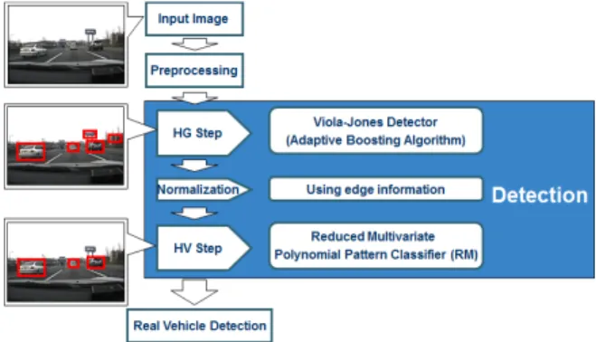
Fig. 1. HG and HV step
In general, a vehicle detection system consists of two basic steps namely, Hypothesis Generation (HG) and Hypothesis Verification (HV) as figure 1[1]. The purpose of the HG step is to find out candidate locations of vehicles. After the HG step,
the HV step is performed to verify the detected candidate vehicles from the HG step.
The HG step can be classified into three categories. First, knowledge-based methods use information which we already known such as symmetry[10], color[11], shadow[12] and corners[13]
information. Second, stereo-based methods take advantage of 3D information such as Inverse Perspective Mapping (IPM)[14] and Disparity Map
[15] but it has the shortcoming of high computational cost. Third, motion-based methods use the information of moving object such as Optical Flow[16]. However, motion-based method can be used for only moving object but it cannot be applied to static object. Recently, many researches try to fuse the results of the HG step to improve the performance.
During the HV step, tests are performed to verify the correctness of a hypothesis from the HG step. In order to get a good performance in HV step, the detection rate should be maintained and the false positive rate has to be greatly decreased from the HG step. The HV step can be classified into two categories. First, template-based methods use predefined patterns from the vehicle class and perfume correlation[17]. Second, appearance-based methods use classifiers which learn the characteristics of the vehicle class from a set of training image[18].
In this paper, we present a novel vehicle detection system using a Reduced Multivariate Polynomial Pattern Classifier (RM)[2] which is easy to implement, and faster but similar performance with SVM. Here, the two basics steps of HG and HV are performed where respectively a Viola and Jones detector (AdaBoost)[3] and a reduced multivariate polynomial pattern classifier (RM) have been adopted. Since SVM has been shown good performance in vehicle detection system[1], the performance of the RM method is finally compared with that of an SVM where both the verification accuracy and the speed of detection are seen to be superior for the proposed RM method.
The rest of this paper is organized as follows.
In section 2, we present the preliminaries of RM[2] for immediate reference. The proposed algorithm is next described in section 3. The results of experiments are presented in section 4.
Finally, some concluding remarks and suggestions for future research are presented in section 5.
Ⅱ. PRELIMINARY: A Reduced Multivariate Polynomial Pattern Classifier[2]
The reduced multivariate polynomial model as seen in [2] can provide an effective way to classify complex nonlinear input-output relationships. Moreover, the method has an advantage of fast processing capability where it can be easily adopted for real-time vehicle detection application with good detection accuracy.
According to [2], the reduced multivariate polynomial model (RM) can be expressed as
⋯
⋯
≥
(1)
where , … are the polynomial inputs,
, , , , … are the weighting coefficients to be estimated, and denote the input-dimension and order of system respectively.
The number of terms in this model can be expressed as :
≈ (2)
The parameters vector can be estimated using
(3)
where is a regularization factor to avoid singularity of , ∈ × denotes the Jacobian matrix of when data points are
given and ∈ is the known inference vector from training data. The selected locations of an image will be classified as either a “vehicle” or a
“non-vehicle”. This is a 2-class classification problem where the target outputs can be set as
“0” for “vehicle” label and “1” for “non-vehicle”
label. Since the output of a trained model is continuous, a threshold process is needed and is adopted as:
(4) The threshold value for classification can be set by train step as the value having the best classification rate.
Ⅲ. THE PROPOSED VEHICLE DETECTION PROCEDURE
For vehicle detection, we follow the above mentioned basic two steps which consist of the HG step and the HV step. In the HG step, the Viola-Jones detector is adopted and in the HV step, a single-output RM is adopted in the HV step. The overall procedure of the proposed vehicle detection scheme is illustrated in Figure 2.
Fig. 2. Flow of the proposed procedure
As seen from Figure 2, an input image is first preprocessed using histogram equalization in order to detect candidate vehicle locations in the HG step. Next, in the HG step, a Viola-Jones detector (AdaBoost)[3] is adopted. Although the Viola-Jones detector has a high detection rate, it has a high probability to recognize non-vehicle region as
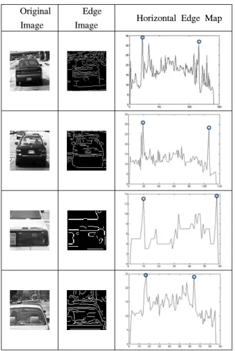
vehicle. Hence, the candidate regions should be verified in the HV step. Subsequently, a normalization step is added between the HG step and the HV step where the detected candidate images are normalized using edge information. In order to find a correct boundary of the vehicle, we construct a vertical and horizontal edge map and find the local maxima. If the local maxima are above a certain threshold, the corresponding coordinates are selected as the boundary. When there are multiple number of local maxima, we select those boundaries which are nearest to the edge of detected regions. This is because most detected regions by the Viola-Jones detector included not only real vehicles but also redundant background edge information. Our selection of boundaries nearest to the region edge can remove such redundant background edge information.
Based on the selected boundaries, the image is further normalized to a size 32×32. Figure 3 shows some sample images for normalization.
Next, the Principal Component Analysis (PCA) method is used to extract relevant features as the input of classifier. Finally, the RM is used as the classifier to obtain the final decision.
Ⅳ. EXPERIMENTS
For experimentation, we use the Caltech Cars (Rear) dataset[4],which consists of 1,155 rear images of various cars. 2,000 rear images, which consist of 1,000 images from the Caltech dataset and 1,000 images from our dataset taken by an on-board camera under different environments are used as positive images as shown in figure 4.
Another 2,000 negative images based on randomly sampled non-vehicle images such as background, road, and traffic sign are also selected. Since we need to train and test the classifiers (SVM and RM) for 2-fold cross-validation, those above positive (vehicle) and negative (non-vehicle) images are divided into two sets. Each of the training set (DB1) and the test set (DB2) consists of 1,000 positive and 1,000 negative images.
Original Image
Edge
Image Horizontal Edge Map
Fig. 3. First column show a detected original image after applying the HG step. Second column represents edge image by the canny method. Third column represents horizontal edge map. The circles in third column denote selected local maxima for normalization
Fig. 4. The example images under different environments
Two types of experiments have been performed in order to observe the performance and the robustness of the proposed use of RM classifier.
The first experiment consists of only an HV step implementation with manually normalized positive and negative images. This is to assess the performance from an off-line perspective. The second experiment consists of combining the HG
and the HV steps in order to observe the robustness aspects of the entire on-line system.
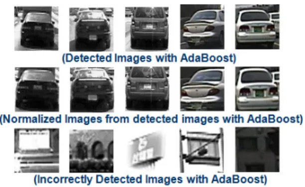
Figure 5 shows some samples of the off-line dataset consisting of manually normalized images for experiment 1 (experiment of the HV step only). Figure 6 shows some image of on-line outputs from AdaBoost detector for experiment 2 (experiment of the HG and HV steps combined).
In other word, experiment 1 is performed to verify and compare the performance as only classifier. Experiment 2 is performed to verify the reliability in actual system which consists of HG and HV step. Therefore, the detected images from HG step are used to input of HV step in experiment 2. In case of experiment 2, a location of non-vehicle can be detected as a location of vehicles incorrectly in HG step, so it need to verify whether the location is real vehicle or not.
Therefore, the negative images of HV step are incorrectly detected images with AdaBoost in experiment 2.
All images are normalized by 32×32 sizes. We reduced the number of feature dimension to 100, 200 and 300 respectively as the input of classifiers, SVM and RM, by PCA. Both experiments have been executed on an AMD Athlon 64 X2 Daul Core Processor 3800+ and Matlab.
Fig. 5. Input test images for the HV step only
Fig. 6. Input test images for the combined HG step and HV step
4.1 Results from the HV step only
In this experiment, we compare the verification performance between RM and SVM. For RM, we have experimented with polynomial orders 1(RM_1), 2(RM_2), and 3(RM_3). Since order 3 shows a saturated performance, the experiment stops at order 3. In the SVM experiments, we adopt a linear model, a polynomial model and a radial basisfunction as kernels. The performance of SVM classifier depends on the number of support vectors. To compare the performance between SVM and RM, we used the number of support vector which has the best performance with respect to the speed and classification rate.
To reduce the impact of convergence from different parameters, the SVMs were trained 10 times using different cost parameter C and the average test results were recorded. The average number of support vectors in each class was found to be [252, 253], [253, 252] and [253, 253] ([support vectors from class1 (vehicle), support vectors from class2 (non-vehicle)]) respectively when the number of PCA features were 100, 200 and 300. We performed the 2-fold cross validation by using DB1 and DB2.
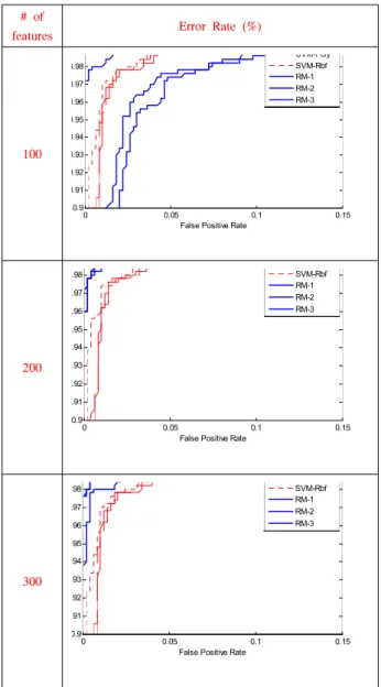
Figure 7 shows the Receiver Operating Characteristic (ROC) curve. Table 1 shows the equal error rates (EER) for SVM (adopting different kernels) and RM (at different polynomial orders) at experimented feature sizes. Here, we see that the RM classifier shows a better performance than that of SVM for all feature sizes. Regarding the processing speed, test CPU
# of Features
SVM Linear
SVM Poly
SVM Rbf
RM 1
RM 2
RM 3 100 0.030 0.032 0.030 0.008 0.012 0.008 200 0.028 0.030 0.026 0.012 0.016 0.010 300 0.028 0.028 0.026 0.010 0.012 0.008 Table 1. EER of HV step only
time for evaluating all test samples, as shown in figure 8, the RM classifier shows a faster speed than SVM. The off-line performance of RM classifier is hence seen to be better than that of the SVM classifier in this experiment.
# of
features Error Rate (%)
100
0 0.05 0.1 0.15
0.9 0.91 0.92 0.93 0.94 0.95 0.96 0.97 0.98
False Positive Rate
SVM-Poly SVM-Rbf RM-1 RM-2 RM-3
200
0 0.05 0.1 0.15
0.9 .91 .92 .93 .94 .95 .96 .97 .98
False Positive Rate
SVM Poly SVM-Rbf RM-1 RM-2 RM-3
300
0 0.05 0.1 0.15
0.9 0.91 0.92 0.93 0.94 0.95 0.96 0.97 0.98
False Positive Rate
y SVM-Rbf RM-1 RM-2 RM-3
Fig. 7. Experimental Results: ROC curve of HV step only
Fig. 8. Experimental Results: Processing time of HV step only. The blue, green and red bar represents that the number of features is 100, 200 and 300 respectively
4.2 Results from the HG and HV step combined
An AdaBoost detector is developed for the HG step in this experiment. As for the Viola-Jones detector, we adopted an implementation from OpenCV[20], which is a library for real time computer vision by Intel. We train a strong classifier based the AdaBoost algorithm using a Harr-like feature based on 400 positive images (150 images from ‘Cars 1999 dataset, CALTECH’
and 250 images from our dataset) and 700 negative images which are randomly sampled from non-vehicle images such as background, road and traffic sign. Each image is sized at 128x128.
Based on DB1 and DB2, the AdaBoost detector detects correctly 91.6% of the positive images with 6.4% of the negative images detected as vehicle regions.
The detected regions are normalized based on the above mentioned normalization procedure.
Figure 5 shows an example of the detected regions using the AdaBoost detector, and normalized regions. In order to evaluate the accuracy of boundary position, we compare the top-left and bottom-right coordinates of normalization results with the ground truth (measured manually) in terms of the mean squared error (MSE). Since the detected region is square, we used the top-left and bottom-right
coordinates to compare. MSE can be expressed as:
(5)
where, denotes estimated coordinates from normalization and is ground truth coordinates.
Table 2 shows the evaluation result of the normalization step.
Top-left Bottom-right
With normalization
Without normalization
With normalization
Without normalization
MSE 2435.2 3716.8 2903.4 4071.6
Table 2. Evaluation result for the accuracy of the normalization step
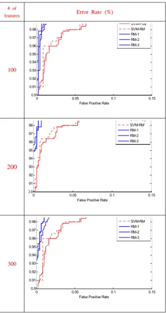
The normalized 1,832 positive images and 128 negative images from the HG step are verified in the HV step. Figure 9 shows the performance of HG+HV step in terms of ROC curves. In addition, to show the effectiveness of normalization step, we compare the detection performance by normalization with that without normalization in terms of the equal error rate in Table 3. These overall results are seen to have a higher error rate than those using only the HV step. This is because the detected regions from AdaBoost in the HG step contain some redundancy even though normalization step is applied before the HV step. In this experiment, the RM classifier is seen to have better performance than SVM classifier.
In real-time systems, the processing time per frame is important. Table 4 shows the processing time for each process. It takes 39.8, 39.9 and 40.1 msec for total processing time for a frame respectively by RM_1, RM_2 and RM_3.
Therefore, the system can be operated in 25 frames/sec. Although a fast processing speed is important, a reliable estimation is more important since it is related to safety in automotive driver assistance systems. Therefore, considering both results of ROC and speed from this experiment, the performance of a 3rd order RM when the number of features is 300 shows the most reliable
performance in this experiment.
# of
features Error Rate (%)
100
0 0.05 0.1 0.15
0.9 0.91 0.92 0.93 0.94 0.95 0.96 0.97 0.98
False Positive Rate
SVM-Poly SVM-Rbf RM-1 RM-2 RM-3
200
0 0.05 0.1 0.15
0.9 .91 .92 .93 .94 .95 .96 .97 .98
False Positive Rate
SVM-Rbf RM-1 RM-2 RM-3
300
0 0.05 0.1 0.15
0.9 .91 .92 .93 .94 .95 .96 .97 .98
False Positive Rate
SVM-Rbf RM-1 RM-2 RM-3
Fig. 9. Experimental Results: ROC curve of HG + HV steps combined
# of feature Classifier
100 200 300
W/O W W/O W W/O W
SVM Linear 0.044 0.028 0.046 0.026 0.044 0.026 SVM Poly 0.044 0.024 0.042 0.022 0.042 0.022 SVM Rbf 0.042 0.022 0.042 0.020 0.048 0.020 RM_1 0.048 0.016 0.042 0.034 0.042 0.042 RM_2 0.044 0.012 0.040 0.018 0.048 0.012 RM_3 0.044 0.014 0.038 0.012 0.038 0.012
Table 3. EER of HG + HV steps combined. W: with and W/O: without
Content Processing time / frame (msec)
Read a frame 8.60
Preprocessing (convert color to
gray, Histogram equalization) 0.53 Viola-Jones detector 12.78
Normalization 17.62
Verification : RM1 RM2 RM3
0.24 0.37 0.58 Table 4. Processing time per frame in the system
Ⅴ. CONCLUSION
For robust vehicle detection, a detection system which consists of a HG step and a HV step has been proposed. From the experiments, the adopted RM classifier shows a better performance in terms of accuracy and processing speed compared with the SVM classifier. Moreover, the RM is seen to be robust to the variation of input vehicle region when the HV step is combined with the HG step using an AdaBoost detector when the number of features is sufficient. The RM classifier is thus perceived to be an effective tool for real-time vehicle detection system development. Our future work includes development of an even more robust system considering various adverse conditions in the training and testing processes.
REFERENCES
[1] Z. Sun, G. Bebis and R. Miller, “On-road vehicle detection: a review,” IEEE Trans.
Pattern Anal. Mach. Intell., 28(5), pp. 694-711, 2006.
[2] K.A. Toh, Q.L. Tran and D. Srinivasan,
“Benchmarking a Reduced Multivariate Polynormial Pattern Classifier,” IEEE Trans.
Pattern Anal. Mach. Intell., 26(6), pp. 740-755, 2004.
[3] P. Viola and M. J. Jones, “Rapid Object Detection using a Boosted Cascade of Simple Features,” in Proc. the IEEE conf. on Computer Vision and Pattern Recognition, 1(2), pp.
511-518, 2001.
[4] Caltech datasets are from
http://www.robots.ox.ac.uk/∼vgg/data/
[5] O. Nakayama, M. Shiohara, S Sasaki, T Takashima and D Ueno, “Robust Vehicle Detection under Poor Environmental Conditions for Rear and Side Surveillance,” IEICE Transactions on Information and System, E87-D(1), pp. 97-104, 2004.
[6] A. Giachetti, M. Campani, and V. Torre, “The Use of Optical Flow for Road Navigation,”
IEEE Trans. Robotics and Automation, 14(1), pp. 34-48, 1998.
[7] Z. Sun, G. Bebis and R. Miller, “Improving the performance of on-road vehicle detection by combining Gabor and wavelet features,” in Proc. the IEEE conf. on Intelligent Transportation Systems, pp. 130–135, 2002.
[8] N. Matthews, P. An, D. Charnley, and C.
Harris, “Vehicle Detection and Recognition in Greyscale Imagery,” Control Engineering Practice, 4(4), pp. 473-479, 1996.
[9] Ju-Hyun Cho and Seogn-Dae Kim, “Object detection using multi-resolution mosaic in image sequences,” Signal Processing : Image Communication, 20(3), pp. 233-253, 2005.
[10] A. Kuehnle, “Symmetry-Based Recognition for Vehicle Rears,” Pattern Recognition Letters, 12(4), pp. 249-258, 1991.
[11] J.C. Rojas and J.D. Crisman, “Vehicle detection in color images,” in Proc. the IEEE conf. on Intelligent Transportation System, pp. 403-408, 1997.
[12] C. Tzomakas and W. Seelen, “Vehicle Detection in Traffic Scenes Using Shadows,”
Technical Report 98-06, Institut fur Neuroinformatik, Ruht-Universitat, Bochum, Germany, 1998.
[13] M. Bertozzi, A. Broggi, and S. Castelluccio, “A Real-Time Oriented System for Vehicle Detection,” Journal of Systems Architecture, pp.
317-325, 1997.
[14] H. Mallot, H. Bulthoff, J. Little, and S. Bohrer,
“Inverse Perspective Mapping Simplifies Optical Flow Computation and Obstacle
Detection,” Biological Cybernetics, 64(3), pp.
177-185, 1991.
[15] R. Labayrade and D. Aubert, “In-vehicle obstacles detection and characterization by stereovision,” in Proc. the 1st Workshop on In-Vehicle Cognitive Computer Vision Systems, 2003.
[16] A. Giachetti, M. Campani, and V. Torre, “The Use of Optical Flow for Road Navigation,”
IEEE Trans. Robotics and Automation, 14(1), pp. 34-48, 1998.
[17] A. Bensrhair, M. Bertozzi, A. Broggi, P. Miche, S. Mousset, and G. Moulminet, “A Cooperative Approach to Vision-Based Vehicle Detection,”
in Proc. the IEEE Conf. on Intelligent Transportation Systems, pp. 209-214, 2001.
[18] Z. Sun, R. Miller, G. Bebis and D. DiMeo, “A real-time precrash vehicle detection system”, in Proc. IEEE Int’l Workshop Applications of Coputer Vision, pp. 171-176, 2002.
[19] S. Park, T. Kim, S. Kang, and K. Heon, “A Novel Signal Processing Technique for Vehicle Detection Radar,” 2003 IEEE MTT-S Int’l Microwave Symp. Digest, pp. 607-610, 2003.
[20] Intel OpenCV library is from http://sourceforge.net/ projects/opencvlibrary/
김 중 락 (Joongrock Kim)
2005년 2월 고려대학교 전자 및 정보공학과 학사 2008년 8월 연세대학교 생체 인식협동과정 석사
2008년 9월~현재 연세대학교 전기 전자공학과 박사과정
<관심분야> Object Detection / Tracking, 3D vision, HCI,
유 선 진 (Sunjin Yu)
2003년 8월 고려대학교 전자 및 정보공학과 학사
2006년 2월 연세대학교 생체 인식협동과정 석사
2011년 2월 연세대학교 전기 전자공학과 박사
2011년 1월~2012년 5월 LG 전자 선임연구원
2012년 6월~현재 연세대학교 연구교수
<관심분야> 3D vision, HCI, 얼굴 인식
Kar-Ann Toh
1990년 National University of Singapore 학사
1992년 Nanyang Technological University 석사
1999년 Nanyang Technological University 박사
2005년~현재 연세대학교 전기 전자공학부 교수
<관심분야> biometrics, pattern recognition, optimization, and neural networks.
김 도 훈 (Do-hoon Kim)
1998년 2월 POSTECH 전자 전기공학과 학사
2000년 2월 POSTECH 전자 전기공학과 석사
2010년 3월~현재 연세대학교 전기전자공학부 박사과정 2005년 10월~현재 KETI 무선플랫폼센터 선임연구원
<관심분야> 전자공학, 통신신호처리
이 상 윤 (Sangyoun Lee)
1987년 2월 연세대학교 전자 공학과 학사
1989년 2월 연세대학교 전자 공학과 석사
1999년 2월 Georgia Tech. 전 기 및 컴퓨터공학과 박사 1989년~2004년 KT 선임연구원 2004년~현재 연세대학교 전기전자공학부 부교수
<관심분야> 생체인식, 컴퓨터비전, 영상부호화