IEG 환경지질연구정보센터

전체 글

(1)LANDSLIDE SUSCEPTIBILITY ANALYSIS USING GIS AND ARTIFICIAL NEURAL NETWORK Moung-Jin Lee*, Joong-Sun Won* ,Saro Lee**. Abstract : The purpose of this study is to develop landslide susceptibility analysis techniques using artificial neural network and to apply the newly developed techniques to the study area of Boun in Korea. Landslide locations were identified in the study area from interpretation of aerial photographs, field survey data, and a spatial database of the topography, soil type, timber cover, geology and land use. The landslide-related factors (slope, aspect, curvature, topograhic type, soil texture, soil material, soil drainage, soil effective thickness, timber type, timber age, and timber diameter, timber density, geology and land use) were extracted from the spatial database. Using those factors, landslide susceptibility was analyzed by artificial neural network methods. For this, the weights of each factor were determinated in 3 cases by the backpropagation method, which is a type of artificial neural network method. Then the landslide susceptibility indexes were calculated and the susceptibility maps were made with a GIS program. The results of the landslide susceptibility maps were verified and compared using landslide location data. A GIS was used to efficiently analyze the vast amount of data, and an artificial neural network was turned out be an effective tool to maintain precision and accuracy.. Key words: Landslide, Susceptibility, GIS, Artificial neural network, Weight Moung-Jin Lee*, Joong-Sun Won* 2. Department of Earth System Science, Yonsei University, 134, Shinchondong, Seoul, 120-749,. Korea E-mail: [email protected]. Saro Lee 1. National Geoscience Information Center, Korea Institute of Geology, Mining & Materials. (KIGAM), 30, Kajung-Dong, Yusung-Ku, Taejon, 305-350, Korea E-mail: [email protected].. 1.

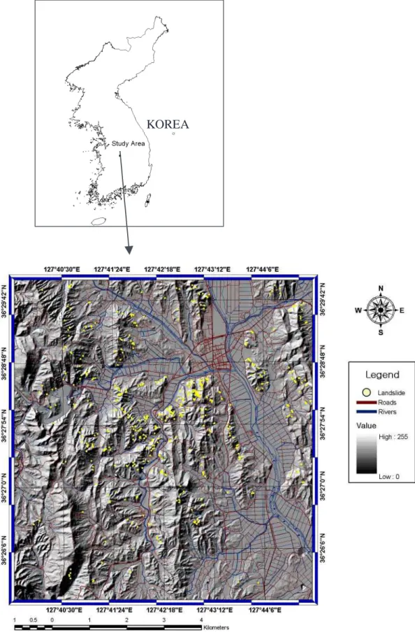
(2) Introduction There are many studies for landslide hazard evaluation using GIS (Larsen and Torres-Sanchez, 1998; Turrini and Visintainer, 1998; Guzzetti and others, 1999; Chung and Fabbri, 1999; Gokceoglu and others, 2000; Fernández and others, 1999; Randall and others, 2000; Luzi and others, 2000; Lee and Min, 2001; Mandy and others, 2001). The Boun area of study had much landslide damage following heavy rain in 1998 and was selected as a suitable case to evaluate the frequency and distribution of landslides (Fig. 1). The site lies between the latitudes 36 °25’ 21’’ N and 36° 30’ 00’’ N, and longitudes 127° 39’ 36’’ E and 127° 45’ 00’’ E, and covers an area of 68.43km2. The bedrock geology of the study area consists mainly of biotite granite. In the study area, the landslides were mainly soil slide that occurred and the landslides occurred where the maximum daily rainfall is 407 mm. The study area had considerable landslide damage following heavy rains in 1998, and was consequently selected as a suitable case to evaluate susceptibility to landslides. For the landslide susceptibility analysis (Fig. 2), first, the study area was selected, then landsliderelated databases were collected, artificial neural network were trained, weights were determinated landslide susceptibility was analyzed, the result was verified, and the landslide susceptibility map was created. Landslide occurrence areas were detected in the study area by interpretation of aerial photography and field survey data (Fig. 1). Landslide location, topography, soil, and forest databases were used for the analysis. Maps constructed in a vector format spatial database using the GIS software ARC/INFO were used for application of artificial neural network methods. These included 1:5,000 scale topographic maps, 1:25,000 scale soil maps, 1:25,000 scale forest maps, 1:50,000 scale geological map and 30m-resolution land use data from TM satellite image. From the maps, 14 factors (slope, aspect, curvature, topograhic type, soil texture, soil material, soil drainage, soil effective thickness, timber type, timber age, and timber diameter, timber density, geology and land use) used for landslide susceptibility analysis were extracted. The landslide susceptibility was analyzed using an artificial neural network program partially modified from the original version developed by Hines (1997) in the MATLAB package. Finally, the analysis forecast was verified using landslide location. For the artificial neural network application for landslide susceptibility analysis, locations of landslide occurrence and non-occurrence were assigned to training areas for supervised classification. When the weights converged to reasonable values, the weight that satisfied the stopping criterion during the training, landslide susceptibility was analyzed using the weights modified by back propagation between neural network layers. Finally, the analysis results were converted to grid data and the landslide susceptibility map was made using GIS.. The benefits of integrating GIS and artificial neural network are efficiency and ease of management, input, display and analysis of spatial data for landslide susceptibility analysis. Moreover, the artificial neural network has many advantages compared with statistical methods. Firstly, the artificial neural network method is independent of the statistical distribution of the data. Therefore, integration of remote sensing data or GIS data is convenient. Benediktsson et al. (1990). 2.

(3) improved classification accuracy using artificial neural network for integration of Landsat MSS imagery and a topographic database (altitude, slope and aspect). Wilkinson (1993) also verified an artificial neural network utilization in a GIS. Secondly, there is no need a specific statistical variable. Thirdly, accurate analysis is possible through training area datasets is a few because of pixel based calculations (Paola and Schowengerdt, 1995). However, resultant values do not accurately coincide with the correct values because of the random initial weights, variables have to be selected empirically, and the execution time is longer than statistical method such as maximum likelihood method.. Artificial neural network An artificial neural network is a “computational mechanism able to acquire, represent, and compute a mapping from multivariate space of information to another, given a set of data representing that mapping” (Garrett, 1994). Artificial neural network is trained by the use of a set of examples of associated input and output values. The purpose of an artificial neural network is to build a model of the data generating process so that the network can generalize and predict outputs from inputs that it has not previously seen. The most frequently used neural network method is the backpropagation-learning algorithm. This is a learning algorithm of multi-layered neural network, which consists of an input layer, hidden layers, and an output layer. The hidden and output layer neurons process their inputs by multiplying each of their inputs by the corresponding weights, summing the product, then processing the sum using a nonlinear transfer function to produce a result. The S-shaped sigmoid function is commonly used as the transfer function. Artificial neural network “learns” by adjusting the weights between the neurons in response to the errors between actual output values and target output values. At the end of this training phase, the neural network represents a model, which should be able to predict a target value given an input value. For use of artificial neural network in a GIS, the GIS spatial database must be converted to the format of input data for the artificial neural network program, and conversely the artificial neural network output data must converted to the format for the GIS spatial database. It is hard to ascertain the actual internal processing in artificial neural network programs, and they consume considerable execution time and computer capacity owing to a large amount of computation. However, artificial neural network models are adaptive and capable of generalization. They can handle imperfect or incomplete data, and can capture nonlinear and complex interactions among variables of a system. There are 3 stages involved in using neural networks for multi-source classification; the training stage, thee determinating weight, and the classification stage. The backpropagation algorithm trains the network, typically, until some targeted minimal error is achieved between the desired and actual output values of the network. Once training is complete, the network is used as a feedforward structure to produce a classification for the entire image (Paola and Schwengerdt, 1995). In this study, we only use a inter-layer weights of training stage. A neural network consists of a number of interconnected nodes. Each node is a simple processing. 3.

(4) element that responds to the weighted inputs it received from other nodes. The arrangement of the nodes is referred to as the network architecture (Fig. 3). The receiving node sums the weighted signals from all nodes to which it is connected in the preceding layer. Formally, the input that a single node receives is weighted according to Eq. (1).. net j =. ∑w ⋅o ij. i. (1). i. where wij represents the weights between node i and node j, and oi is the output from node j such as Eq. (2).. o j = f (net j ). (2). The function f is usually a non-linear sigmoid function that is applied to the weighted sum of inputs before the signal processes to the next layer. Advantage of the sigmoid function is that its derivative can be expressed in terms of the function itself such as Eq. (3).. f ' (net j ) = f (net j )(1 − f (net j )). (3). The Multi-layer Perceptron (MLP) can separate data that are non-linear because it is ‘multi-layer’, and it generally consists of three types of layers. The first layer is the input layer, where the nodes are the elements of a feature vector. The second type of layer is the internal or ‘hidden’ layer since it does not contain output unit. The third type of layer is the output layer and this presents the output data. Each node in the network is interconnected to the nodes in both the preceding and following layers by connections. These connections have associated with them weights (Atkinson and Tatnall, 1997). The error, E, for one input training pattern, t, is a function of the desired output vector, d, and the actual output vector, o, given by Eq. (4).. E=. 1 2. ∑ (d. k. − ok ). (4). k. The error back propagated through neural network and the error is minimized by changing the weight between layer. So, the weight can be expressed in Eq. (5).. wij (n + 1) = η (δ j ⋅ oi ) + α∆wij. (5). Where η is the learning rate parameter, δj is an index of the rate of change of the error, and α is the momentum parameter. This process of feeding forward signals and back propagating the error. 4.

(5) is repeated iteratively until the error of the network as a whole is minimized or reaches an acceptable magnitude. Using the backpropagation, the weight of the each factor can be recognized and the weight can be used to weight of classification. Zhou (1999) described the method of determination of the weight using backpropagation. From Eq. (2), the effect of an output oj a hidden layer node j on the output ok from an output layer node k can be represented by the partial derivative of ok with respect to oj such as Eq. (6). ∂o k ∂(net k ) = f ' (net k ) ⋅ = f ' (net k ) ⋅ w jk ∂o j ∂o j. (6). The Eq. (6) equation can produce values with both positive and negative signs. If only the magnitude of the effects is of interest, the importance of node. j. relative to another node j 0 j0 in. the hidden layer can be calculated as the ratio of the absolute values from the Eq. (6) equation.. ∂o k. ∂o k. /. ∂o j. f ′(net k ) ⋅ w jk. =. ∂o j 0. f ′(net k ) ⋅ w j 0k. =. w jk. (7). w j0k. The Eq. (7) shows that, with respect to a particular node in the output layer, the relative importance of a node in the hidden layer is proportional to the absolute value of the weight on its connection to the node in the output layer. When more than one node in the output layer is concerned, the Eq. (7) equation cannot be used to compare the importance of two nodes in the hidden layer.. w j0k =. t jk =. 1 ⋅ J. ∑w J. j =1. w jk 1 ⋅ J. ∑w. =. J. j =1. (8). jk. jk. J ⋅ w jk. ∑w J. j =1. (9). jk. Therefore, with respect to node k, each node in the hidden layer has a value greater or smaller than one, depending on whether it is more or less important than the average, respectively. With respect to the same node, all the nodes in the hidden layer have a total importance such as Eq. (10),. ∑t J. j =1. jk. =J. (10). 5.

(6) Consequently, with respect to all nodes in the output layer, the overall importance of node j can be calculated as Eq. (11).. ∑t K. 1 ⋅ K. tj =. j =1. (11). jk. Similar to Eq. (11), with respect to node j in the hidden layer, the normalized importance of node j in the input layer can be defined as Eq. (12).. ω ij. s ij =. 1 ⋅ I. =. I ⋅ ω ij. ∑ω ∑ω I. ij. i =1. (12). I. i =1. ij. With respect to the hidden layer, the overall importance of node i is Eq. (13). si =. 1 ⋅ J. ∑s J. j =1. (13). ij. Correspondingly, the overall importance of input node i with respect to output node k is given by Eq. (14).. st i =. 1 ⋅ J. ∑s J. j =1. ij. ⋅t j. (14). Spatial database construction using GIS In the study area, several types of landslides were documented; rainfall-triggered debris flows and shallow soil were the most abundant. The instability factors include lithology and geological structure, bedding altitude, seismicity, slope steepness and morphology, stream evolution, groundwater conditions, climate, vegetation cover, land use, and human activity. The availability of thematic data varies largely, depending on the type, scale, and method of data acquisition. Geomorphologic, lithologic, soil, forest and land-use data should be available for the entire area. A digitized map of landslide boundaries was used, and these digital data were input to the GIS. A vector-to-raster conversion was undertaken to provide a raster data of landslide areas with 10 m × 10 m pixels. To apply the artificial neural network method, a spatial database that took into was considered as landslide-related factors, such as topography, soil, forest, geology and land use, was collected and used. Landslide occurrence areas were detected in the Boun area, Korea, by interpretation of aerial photographs and field survey data. A database was constructed by georectifying and merging many. 6.

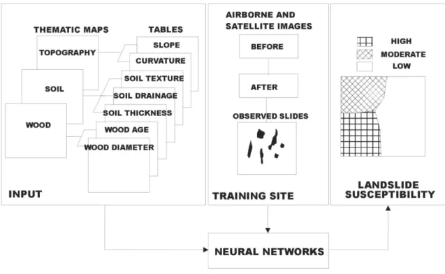
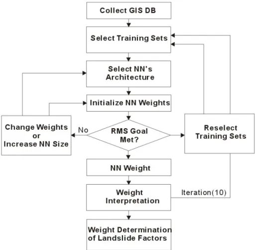
(7) aerial photographs. Topography, soil, forest, and geology databases were also constructed. A map of recent landslides was developed from 1:20,000 scale aerial photography in combination with the GIS, and this was used to evaluate the frequency and distribution of shallow landslides in the area. Maps relevant to landslide occurrence were constructed in a vector format spatial database using the GIS software ARC/INFO. These included 1:5,000 scale topographic maps, 1:25,000 scale soil maps, 1:25,000 scale forest maps, and 1:50,000 scale geological maps. Contour and survey base points that have an elevation value read from the topographic map were extracted, and a DEM (Digital Elevation Model) was made. The DEM has the 10m resolutions. Using the DEM, the slope, aspect and curvature were calculated. Soil texture, parent material, drainage, effective thickness, and topographic type were extracted from the soil database. Forest type, timber age, timber diameter, and timber density were extracted from the forest map. Lithology was extracted from the geological database, and land use was classified from Landsat TM satellite imagery (Table 1). Using the detected landslide locations and the constructed spatial database, a landslide analysis method, with artificial neural network, was applied and verified. To achieve this, the calculated and extracted factors were converted to a 10 m × 10 m grid (ARC/INFO GRID type), and then converted to ASCII data for use with the artificial neural network program. The analysis results were converted to grid data using GIS.. Landslide susceptibility analysis using artificial neural network - Determination of Weight Artificial neural network methods have previously been applied to land use and cover classification using satellite imagery (Schaale and Furrer, 1995; Serpico and Roli, 1995). In particular, the multi-layer perceptron method using the backpropagation algorithm was used widely in a supervised classification with training area data (Atkinson and Tatnall, 1997). The supervised classification is assigned at the site where the information is well known; this training site is classified by analysis of the input data for the site. By this process, landslide susceptibility data were analyzed in this study using artificial neural network methods. Fig. 4 is the flowchart of neural networks training for weight determination. The weight between layers that acquired by training of neural network calculated reversely and the contribution or importance of each factor is calculated. So, the contribution or importance of each factor, Weight, was determinated. A GIS spatial database was used as input data and landslide locations were used as training sites. The constructed landslide related factors do not have a Gaussian distribution and are not statistically related or distributed amongst the supervised classification, so the backpropagation neural network method was used. In the artificial neural network method, the 14 factors were used. The program developed by Hines (1997) using MATLAB was partially modified for the landslide analysis. It was modified in the input and output parts for the use of GIS data. In this analysis, the study area was divided into a 10 m × 10 m pixel grid (ARC/INFO GRID format), which was converted to ASCII format for use in the artificial neural network program. There were 658,790 cells in the study area, and 11,735(1.78 %) of them experienced landslides.. 7.

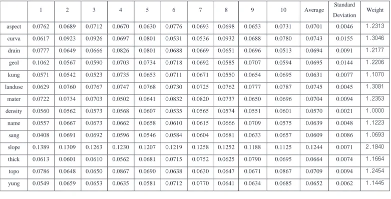
(8) For analysis of landslide susceptibility, the training sites were selected from the landslide-related factors and the backpropagation algorithm was applied to calculate weights between the input layer and the hidden layer, and between the hidden layer and the output layer, by modifying the number of hidden layers and the learning rate. The weights were applied to the entire study area and the landslide susceptibility index value was calculated. The calculated index values were converted into an ARC/INFO GRID using the GIS. Then the landslide susceptibility map was created using the GRID data. A three-layered feed forward network was implemented in MATLAB on the basis of the framework provided by Hines (1997). Feed-forward means that all the interconnections between the layers propagate forward to the next layer (Hines, 1997). The number of hidden layers and the number of nodes in a hidden layer required for a particular classification problem are not easy to deduce. In this study, the structure of 7×15×2 was selected for the network with input data normalized to the range 0.1 to 0.9. The nominal and interval class group data were converted to continuous value between 0.1 and 0.9. The content of the number is not considered in the process of the calculation using neural network program, but the number used for distinguish the classes of each factor in the process of the calculation using artificial neural network program. Therefore, the continuous value is not ordinal data but nominal data, and the numbers mean the classification of the input data. The learning rate was set to be 0.01, and the initial weights were randomly selected. The initial weights were set between 0.1 and 0.3 automatically. To test whether the variation of weights is dependent on initial weight or not, the weights which were calculated from many case, were compared. The result revealed that the initial weight do not have influence on weight in the condition. From each of the two classes (landslide and not-landslide), 200 pixels per class were selected as training pixels randomly. The landslide prone (occurrence) locations and the landslide non-prone locations were selected as training sites. The 10 training sites were selected randomly for influence of the training site and the training sites were processed 10 times iterately for recognized the change of initial weight. From each of these areas, 200, 400, and 600 pixels locations were randomly extracted and analyzed. As a result, the number of training locations did not influence the analysis by much. The selected landslide prone locations were assigned (0.1, 0.9) and the landslide not prone locations were assigned (0.9, 0.1). To lessen the error between the predicted output values and the actually calculated output values, the backpropagation algorithm was used. The algorithm propagates the weights backwards and then controls the weights. The numbers of epochs were set to 1,000 and RMSE (Root Mean Square Error) goal for stopping criterion was set to 0.1. Most of iteration met the 0.1 RMS goal. However, if the goal is not met, the iteration is stopped in the 1000 epochs. In the case, the maximum RMS was under 0.5. After training, the weights were determined, as shown in Table 2, Table 3 and Table 4. The results were repeated 10 times. As the initial weights were assigned random values, the results were not the same. Therefore, in this study, the calculation was repeated 10 times, and the results revealed similar values. The standard deviation is distributed from 0 to 1.1, so the random sampling don’t’ have large effect to the result. For easy interpretation, the average values were calculated, and these values were divided by the weight of the timder density that had a minimum value. As the. 8.

(9) weight has relative importance for each factor, the divided values that were calculated were used. The timder density value used was the minimum value, 1.00, and the topographic slope used was the maximum value, 2.1840. The land use used was 1.3081, and the curvature used was 1.3046. The calculated values were used in the landslide susceptibility analysis, as weights improve the accuracy of the analysis, and can be used as standardization weights.. Conclusions and discussion Landslides are one of the most hazardous natural disasters, not only in Korea but also in worldwide. Government and research institutions worldwide have attempted for years to assess landslide hazards and risks and to show their spatial distribution. An artificial neural network approach to estimating the areas susceptible to landslides using a spatial database (SDB) is presented. For the landslide susceptibility analysis, a landslide location SDB and a landsliderelated database was constructed for the study area of Yongin, in Korea. In the study area, landslide occurrence locations detected from aerial photograph interpretation and field survey data were formed into a GIS database. From the spatial DB, landslide-related factors were calculated and extracted. The factors involved are slope and curvature (derived from the topography database); soil texture, drainage, and effective thickness (from the soil database); and trunk diameter and stand age (from the forest database). Using these seven factors, artificial neural network methods were applied to analyze the landslide susceptibility. For application of the artificial neural network methods, the training sites were selected from landslide-related factors, and a backpropagation algorithm was applied to calculate weights between input layers and hidden layers and between hidden layers and output layers by modifying the number of hidden layers and the learning rate. The weights were applied to the entire study area, and a landslide susceptibility map was made. The result of the analysis (the forecast) was used to construct a GIS layer, and it was mapped. This was verified by calculating the correlation observed between actual landslide occurrence location and the forecast. The result of the verification was a satisfactory agreement between the susceptibility map and the landslide location data. In this neural network method, it is difficult to follow the internal processes of the procedure, and the method entails a long execution time and has a heavy computing load. There is a need to convert the database to another format, such as ASCII; the method requires data be converted to ASCII for use in the artificial neural network program and later reconverted to incorporate it into a GIS layer. Moreover, the large amount of data in the numerous layers in the target area cannot be processed in artificial neural network programs quickly and easily. Using the forecast data, landslide occurrence potential can be assessed, but the landslide events cannot be predicted. However, landslide susceptibility can be analyzed qualitatively, and there are many advantages, such as a multi-faceted approach to a solution, extraction of a good result for a complex problem, and continuous and discrete data processing. To capitalize on these advantages, the artificial neural network methods have to be improved by further application and upgrading of the programs. The landslide susceptibility maps made from the susceptibility index values are of great help to planners and engineers for choosing suitable locations to undertake projects. The results can be. 9.

(10) used as basic data to assist slope management and land-use planning. The methods used in the study are valid for generalized planning and assessment purposes; however, they may be less useful at the site-specific scale where local geological and geographic heterogeneities may prevail. For the method to be more generally applicable, more landslide data are needed, as well as the program being applied to more regions.. 10.

(11) References Atkinson PM, Tatnall ARL. 1997. Introduction neural networks in remote sensing. International Journal of Remote Sensing 18(4): 699-709. Benediktsson JA, Swain PH, Ersoy OK. 1990. Multisource data classification and feature extraction with neural networks. IEEE Transaction on Geoscience and Remote Sensing 28: 540552. Chung CF, Fabbri AG. 1999. Probabilistic prediction models for landslide hazard mapping. Photogrammetric Engineering & Remote Sensing 65(12): 1389-1399. Fernández, CI, Castillo TF, Hamdouni RE, Montero. JC. 1999. Verification of landslide susceptibility mapping: a case study. Earth Surface Processes and Landforms 24(6): 537-544 Garrett J. 1994. Where and why artificial neural networks are applicable in civil engineering. Journal of Computing Civil Engineering 8(2): 129-30. Gokceoglu C, Sonmez H, Ercanoglu M. 2000. Discontinuity controlled probabilistic slope failure risk maps of the Altindag (settlement) region in Turkey. Engineering Geology 55: 277–296. Guzzetti F, Carrarra A, Cardinali M, Reichenbach P. 1999. Landslide hazard evaluation: a review of current techniques and their application in a multi-scale study. Central Italy. Geomorphology 31: 181-216. Hines JW. 1997. Fuzzy and Neural Approaches in engineering. John Wiley and Sons, Inc. New York: 210 Larsen M. , Torres-Sanchez A. 1998. The frequency and distribution of recent landslides in three montane tropical regions of Puerto Rico. Geomorphology 24: 309-331. Lee, S. 1998. Analysis of Landslide Susceptibility in Korea using Geographic Information System. Proceedings of International Symposium on Application of Remote Sensing and Geographic Information System to Disaster Reduction, Tsukuba, Japan. 141-147. Lee S. Min K. 2001. Statistical analysis of landslide susceptibility at Yongin, Korea. Environmental Geology 40: 1095-1113. Luzi L. Pergalani F. Terlien MTJ. 2000. Slope vulnerability to earthquakes at subregional scale, using probabilistic techniques and geographic information systems. Engineering Geology 58: 313– 336. Mandy LG, Andrew MW, Richard A, Stephan GC. 2001. Assessing landslide potential using GIS, soil wetness modeling and topographic attributes, Payette River, Idaho. Geomorphology 37: 149– 165. Randall WJ, Edwin LH, John AM. 2000. A method for producing digital probabilistic seismic landslide hazard maps. Engineering Geology 58: 271–289. Paola JD. Schowengerdt RA. 1995. A review and analysis of backpropagation neural networks for classification of remotely sensed multi-spectral imagery. International Journal of Remote Sensing. 11.

(12) 16(16): 3033-3058. Park Y, Kim K, Yeo W. 1993. A study on Yongin-Ansung landslides in 1991 (in Korean). Korean Geotechnical Journal 9(4): 103-116. Schaale M, Furrer R. 1995. Land surface classification by neural networks. International Journal of Remote Sensing 16(16): 3003-3031. Serpico SB, Roli F. 1995. Classification of multisensor remote-sensing images by structured neural network. IEEE Transaction on Geoscience and Remote Sensing 33: 562-578. Turrini MC., Visintainer P, 1998. Proposal of a method to define areas of landslide hazard and application to an area of the Dolomites, Italy. Engineering Geology 50: 255-265. Wilkinson GG. 1993. The generalization of satellite-derived thematic maps for GIS input. GeoInformations-Systems 6: 24-29. Wang J, Rahman MS. 1999. A neural network model for liquefaction-induced horizontal ground displacement. Soil Dynamics and Earthquake Engineering 18: 555–568.. 12.

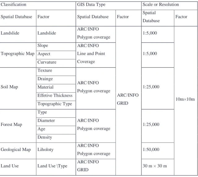
(13) Table 1. Data layer of study area. Classification. GIS Data Type. Spatial Database. Factor. Landslide. Landslide Slope. Topographic Map Aspect Curvature. Spatial Database. Scale or Resolution Factor. ARC/INFO. Spatial Database. Factor. 1:5,000. Polygon coverage ARC/INFO Line and Point. 1:5,000. Coverage. Texture Drainge Soil Map. Material. ARC/INFO. 1:25,000. Polygon coverage. Effetive Thickness. ARC/INFO. Topographic Type. GRID. 10m×10m. Type Forest Map. Diameter. ARC/INFO. Age. Polygon coverage. 1:25,000. Density Geological Map. Liholoty. Land Use. Land Use \Type. ARC/INFO Polygon coverage ARC/INFO GRID. 1:50,000. 30 m × 30 m. 13.

(14) Table 2. Weights of each factor in case 1. Standard. Weightࣜ. 1. 2. 3. 4. 5. 6. 7. 8. 9. 10. Average. aspect. 0.0762. 0.0689. 0.0712. 0.0670. 0.0630. 0.0776. 0.0693. 0.0698. 0.0653. 0.0731. 0.0701. 0.0046. ࣭࣮࣯࣭࣯࣪ࣜࣜ. curva. 0.0617. 0.0923. 0.0926. 0.0697. 0.0801. 0.0531. 0.0536. 0.0932. 0.0688. 0.0780. 0.0743. 0.0155. ࣰࣲ࣭࣯࣪࣬ࣜࣜ. drain. 0.0777. 0.0649. 0.0666. 0.0826. 0.0801. 0.0688. 0.0669. 0.0651. 0.0696. 0.0513. 0.0694. 0.0091. ࣭࣮࣭࣪ࣳࣳࣜࣜ. geol. 0.1062. 0.0567. 0.0590. 0.0703. 0.0734. 0.0718. 0.0692. 0.0585. 0.0707. 0.0594. 0.0695. 0.0144. ࣲ࣭࣮࣮࣪࣬ࣜࣜ. kung. 0.0571. 0.0542. 0.0523. 0.0735. 0.0653. 0.0711. 0.0671. 0.0550. 0.0654. 0.0695. 0.0631. 0.0077. ࣭࣭࣪࣬ࣳ࣬ࣜࣜ. landuse. 0.0629. 0.0760. 0.0767. 0.0747. 0.0768. 0.0730. 0.0725. 0.0762. 0.0777. 0.0787. 0.0745. 0.0045. ࣭࣯࣭࣪࣬ࣴࣜࣜ. mater. 0.0722. 0.0734. 0.0703. 0.0502. 0.0641. 0.0832. 0.0820. 0.0737. 0.0650. 0.0696. 0.0704. 0.0094. ࣱ࣭࣮࣯࣯࣪ࣜࣜ. density. 0.0560. 0.0562. 0.0573. 0.0568. 0.0607. 0.0535. 0.0565. 0.0574. 0.0551. 0.0601. 0.0570. 0.0021. ࣭࣪࣬࣬࣬࣬ࣜࣜ. name. 0.0557. 0.0667. 0.0673. 0.0662. 0.0658. 0.0610. 0.0615. 0.0666. 0.0709. 0.0575. 0.0639. 0.0048. ࣭࣭࣮࣮࣯࣪ࣜࣜ. sang. 0.0408. 0.0691. 0.0692. 0.0596. 0.0546. 0.0584. 0.0604. 0.0681. 0.0633. 0.0657. 0.0609. 0.0086. ࣲ࣭࣯࣪࣬ࣵࣜࣜ. slope. 0.1389. 0.1309. 0.1263. 0.1230. 0.1207. 0.1219. 0.1258. 0.1252. 0.1188. 0.1125. 0.1244. 0.0071. ࣰ࣮࣭࣪ࣴ࣬ࣜࣜ. thick. 0.0613. 0.0601. 0.0610. 0.0562. 0.0681. 0.0715. 0.0752. 0.0625. 0.0790. 0.0695. 0.0664. 0.0074. ࣰࣲࣲ࣭࣭࣪ࣜࣜ. topo. 0.0786. 0.0648. 0.0650. 0.0867. 0.0690. 0.0638. 0.0630. 0.0647. 0.0671. 0.0867. 0.0709. 0.0094. ࣰࣰࣱ࣭࣮࣪ࣜࣜ. yung. 0.0549. 0.0659. 0.0653. 0.0635. 0.0581. 0.0712. 0.0770. 0.0641. 0.0634. 0.0685. 0.0652. 0.0062. ࣰࣰࣱ࣭࣭࣪ࣜࣜ. Deviation. Table 3. Weights of each factor in case 2 Standard. 1. 2. 3. 4. 5. 6. 7. 8. 9. 10. Average. aspect. 0.0841. 0.1021. 0.1170. 0.0992. 0.1196. 0.1251. 0.1245. 0.1065. 0.0828. 0.1088. 0.1070. 0.0153. 1.1020. curva. 0.1193. 0.0946. 0.0722. 0.1156. 0.0976. 0.1065. 0.1110. 0.1021. 0.0967. 0.1001. 0.1016. 0.0132. 1.0465. drain. 0.1033. 0.0857. 0.1356. 0.1005. 0.0971. 0.0971. 0.0646. 0.1339. 0.1361. 0.0878. 0.1042. 0.0240. 1.0732. geol. 0.1173. 0.1060. 0.1199. 0.1058. 0.0965. 0.1258. 0.1252. 0.1063. 0.1385. 0.1169. 0.1158. 0.0124. 1.1933. landuse. 0.1251. 0.0824. 0.0903. 0.1162. 0.0733. 0.0855. 0.0970. 0.0836. 0.1153. 0.1019. 0.0971. 0.0171. 1.0000. mater. 0.1141. 0.0975. 0.1143. 0.0728. 0.1064. 0.0883. 0.0907. 0.1339. 0.0913. 0.1202. 0.1029. 0.0181. 1.0606. slope. 0.2160. 0.2997. 0.2379. 0.2747. 0.3005. 0.2666. 0.2418. 0.2413. 0.2335. 0.2506. 0.2563. 0.0283. 2.6401. topo. 0.1209. 0.1319. 0.1130. 0.1154. 0.1090. 0.1051. 0.1451. 0.0924. 0.1058. 0.1139. 0.1152. 0.0147. 1.1872. Deviation. Weight. Table 4. Weights of each factor in case 3.. aspect. Standard. 1. 2. 3. 4. 5. 6. 7. 8. 9. 10. Average. 0.1236. 0.2322. 0.1805. 0.1685. 0.1268. 0.1568. 0.1875. 0.1609. 0.0932. 0.1642. 0.1594. 0.0386. 1.0000. Deviation. Weight. geol. 0.1446. 0.1330. 0.1648. 0.2668. 0.2105. 0.1426. 0.1833. 0.1235. 0.2436. 0.1380. 0.1751. 0.0498. 1.0983. slope. 0.5619. 0.4038. 0.4886. 0.4007. 0.4951. 0.5429. 0.4684. 0.5247. 0.5041. 0.5304. 0.4921. 0.0546. 3.0868. topo. 0.1699. 0.2310. 0.1660. 0.1640. 0.1676. 0.1577. 0.1608. 0.1909. 0.1592. 0.1674. 0.1734. 0.0222. 1.0881. 14.

(15) KOREA. Fig. 1. Landslide location with hillshaded map.. 15.

(16) Fig. 2. Study flow. Fig. 3. Architecture of artificial neural network. 16.

(17) Fig. 4. Schematic diagram of weight determination for landslide factors using neural network.. 17.

(18)