1
OPTIMAL ROUTE DETERMINATION TECHNOLOGY BASED ON TRAJECTORY QUERYING MOVING OBJECT DATABASE
Kyoung-Wook Min, Ju-Wan Kim, Jong-Hyun Park
LBS Research Team, Telematics Research Group, Telematics&USN Research Division, ETRI 161 Gajeong-dong, Yuseong-gu, Daejeon, 305-350 KOREA
[email protected], [email protected], [email protected]
ABSTRACT:
The LBS (Location-Based Services) are valuable information services combined the location of moving object with various contents such as map, POI (Point of Interest), route and so on. The must general service of LBS is route determination service and its applicable parts are FMS (Fleet Management System), travel advisory system and mobile navigation system. The core function of route determination service is determination of optimal route from source to destination in various environments. The MODB (Moving Object Database) system, core part of LBS composition systems, is able to manage current or past location information of moving object and massive trajectory information stored in MODB is value-added data in CRM, ERP and data mining part. Also this past trajectory information can be helpful to determine optimal route. In this paper, we suggest methods to determine optimal route by querying past trajectory information in MODB system and verify the effectiveness of suggested method.
KEY WORDS: Location-based Service, Moving Object Database, Trajectory, Route
1. INTRODUCTION
In location-based services, the location is defined as location value of movable object such as mobile handset, telematics terminal and mobile station. And this moving object data is very large volume in any LBS application.
So, there are some needs that management, fast retrieve from huge historical moving object dataset. So, the MODB system must be able to manage very large of current location of all moving object and past trajectory which larger than size of current location of object. Also, this MODB system must provide retrieving function which can extract historical object were some area, in some time. The original source of this moving object must be location of navigation application, mobile handset, and terminal of fleet management system and so on. The navigation application can determine route from source to destination where user want to go to, maybe.
And application guides user through that route pass. In generally, the route determination algorithm is depends on the static road network data. That is to say, the route is calculated to pass the fastest time just using value of limited speed of road segment or other static attributes.
So in this paper, we suggest optimal route determination method not as calculating static algorithm but as analyzing real experiential routes of the past. Firstly, we will discuss the problems of the static route determination algorithm. Then, we will explain the overall system architecture to implement the suggested method. And next part, we explain the detailed process of the suggested method. Finally, we will conclude by giving direction for future work.
2. PROBLEM STATEMENT
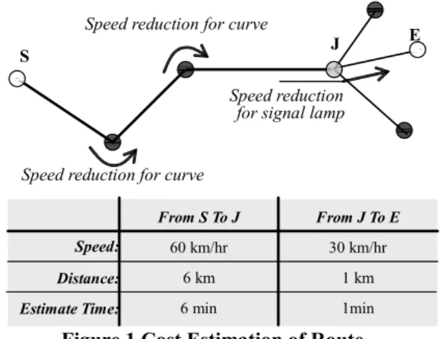
The shortest path algorithm or other deterministic route algorithm is dependent on static road network data. In Figure 1, for example, the function of calculating the route from S to E is executed, the result is like below.
ROUTE route = GetRoute(S, E, RoadNetwork);
Maybe, result route is S→J→E and route.Distance is 7km and route.PassTime is 7 minutes.
Speed reduction for curve S
Speed reduction for curve E
Speed reduction for signal lamp
From S To J 60 km/hr
Estimate Time:
J
From J To E Speed:
Distance:
30 km/hr
6 km 1 km
6 min 1min
Figure 1 Cost Estimation of Route
But, this result of function GetRoute just takes into account each road segment attribute such as max speed, segment length and so on. And, generally, speed of vehicle is reduced in the curved road and at signal lamp of the junction. So, the result pass time, 7 minutes, is not probable and we can guess that the real pass time takes longer than pass time of algorithm result.
We can the pass time driving through route from S to E in practical state; result is described in Table 1. We can easily realize that the pass time is difference as time frame such as rush hour. If the data which is set of information of past moving route like as time stamp at some location, are stored in the repository, then that data are more useful and can provide correctness to determine the rout for navigation.
2 Table 1 Cost of route[S, E] in real world
Pass time from S to E in real world
Car ID Stime stamp Etime stamp Pass Time[S,E]
A001 08:00 08:15 15 min A003 14:13 14:25 12 min B001 15:59 16:09 10 min C001 18:20 18:33 13 min C002 21:09 21:18 9 min
3. ARCHITECTURE
In this paper, we suggest the method provided more useful and more correct route information for travelling through some route using past trajectory of moving object.
It is possible to querying moving object database to get past trajectory of moving object.
Buffer for Trajectory Optimal Routing Analyzer
Moving Object DBMS
Trajectory Road Network
Spatial DBMS
Application layer
Route Analysis Layer
Database Layer Buffer for
Route
Quering Trajectory Quering Route
Request Optimal Route for Navigation
Reporting Location Hand Terminal (Navigation)
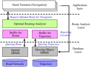
Figure 2 System Architecture
Overall system architecture is in Figure 2. The system is consisting of 3 layer, database layer, route analysis layer, application layer. In the database layer, to determine route by static algorithm, the road network data are managed in the spatial DBMS and to query past trajectory , the moving object data are managed in the moving object DBMS. The route analysis layer, optimal routing analyzer analysis route result by deterministic algorithm and past trajectory result by querying moving object DBMS using analysis factors. The Application layer request optimal route for navigation and must report its location acquired by GPS receiver to moving object DBMS.
3.1 Data Model
In above architecture, road network and moving object are very important basic data which we can determine optimal route analyzing using by and additional analysis factor. We will explain analysis factor in detail in chapter 4.3.
Road Network
The representation of a road network is given by a two-tuple RN = (S, N), where S is set of segment and N is a set of connection node.
Segment
We define a road segment as (ns, ne, list of intermediate point, prop). More specifically, ns is start node, ne is end node, where ns ≠ ne. The geographic information of segment is composed of ns, ne, and list of intermediate point. The properties are length, max speed, min speed, and connected links.
Node
We define a node as (p, prop). Specifically, p = (x, y), prop is a set of connected link.
Moving Object
The representation of a moving object is given by (p, time, velocity, and segment). The p is coordinates as location and time when and segment in which it had been.
Trajectory
The representation of a trajectory is given by (MBRT, list of moving object). The MBRT is minimum bounding rectangle and time period covered all list of moving object, given by (x1, y1, x2, y2, from, to)
3.2 Moving Object Database
The moving object database can be interfacing external client with moql (moving object query language) - sql like format. And there are several components, query processing, buffer management, location index, storage.
In this paper, we exclude detailed structure and function of moving object database. We just query trajectory that has list of consecutive moving object to moving object database. The moving object database can apply various functions; example query is like Figure 3. The examples are finding some car which had been some area and some time; time stamp in first, time slice in second.
Find car which were within 1km from point (x,y) at time t.
SELECT ID FROM FLEETTABLE
WHERE WITHINS(SNAPSHOT(location,t), BUFFER(MPOINT(x, y), 1000) ) = TRUE;
Find car which were within 1km from point (x,y) between time t1 and t2.
SELECT ID FROM FLEETTABLE
WHERE WITHINS(SLICE(location,t1,t2), BUFFER(MPOINT(x, y), 1000) ) = TRUE;
Figure 3 Example of moving object query
4. OPTIMAL ROUTE DETERMINATION MODEL In this chapter, we explain the process of optimal route determination methodology. In the first place, we describe the process of acquisition of GPS device and reporting position in the client side, and then update it to moving object database in the server side.
4.1 The process of report and update position process Client Side Process Scenario
The client system like mobile handset of telematics terminal has main role of acquiring its location and reporting it to moving object database. A series of process is like below;
(1) Pbefore ← Ø (2) do
(3) Pgps ← GetGPS()
(4) Pcurrent ← CoordinateTransformation(Pgps, CoordType)
3 (5) P.segment ← GetSegment(Pcurrent, RN)
(6) if Pcurrent.segment ≠ Pbefore.segment then Report(Pcurrent) (7) Pbefore ← Pcurrent
(8) while sleep()
The case of reporting position to server is acquisition position is on the segment where position of before time is not, like Figure 4.
After client get GPS position, reports it to MODB After client get GPS position, does not report it to MODB
Segment 001 Segment 002
Figure 4 The case of report position to server Server Side Process Scenario
After report position to server side, moving object database store that position executing below query statement.
INSERT INTO table (position.ID, position.x, position.y, position.time, position.velocity, position.segment);
4.2 Extract Road Segment from Trajectory
Just, trajectory information resulted by querying can not calculate distance correctly because trajectory has a list of past position of some moving object. That is to say, past moving position is not continuous but discrete, so sum of moving position distance is Euclidean distance. We must be able to calculate real distance, road segment distance as matching past moving position with segment.
S1
Trajectory View, Euclidean distance Segment View, Road network distance
S2
S3
S4
Figure 5 Trajectory view vs segment view We can calculate real moving distance and real pass time of some moving object from that’s trajectory like below processing.
(1) distance ← Ø, passTime ← Ø (2) for each mo trajectory do
(3) segment ← GetSegment(mo.segment, RN) (4) distance += segment.length
(5) passTime.from ← trajectory.MBRT.from (6) passTime.to ← trajectory.MBRT.to
4.3 Optimal Route Determination Analysis
To determine the route for travelling, source and destination location must be defined. In the static algorithm, shortest route is determined and that’s result is route information that is geometrical polyline and total
distance and estimated pass time. To analyze this route with trajectory, we query moving object database which find moving object to have passed through from the source area to destination area and reverse is possible.
Figure 6 shows this trajectory query statement. The second query is time slice added to before one.
Find car which passed through from the region A to B SELECT ID, POSITION
FROM FLEETTABLE
WHERE PASSES(POSITION, POLYGON(region A)) = TRUE AND PASSES(POSITION, POLYGON(region B)) = TRUE;
Find car which passed through from the region A to B between time t1 and t2
SELECT ID, POSITION FROM FLEETTABLE
WHERE PASSES(POSITION, MPOLYGON(t1, t2, region A)) = TRUE AND PASSES(POSITION, MPOLYGON(t1, t2, region B)) = TRUE;
Figure 6 Trajectory query statement
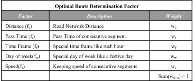
The query result trajectories are candidate routes which are analyzed with static route which is result of deterministic algorithm. We compare static route with trajectories focus on ORDF(Optimal Route Determination Factors). The ORDF is very important to determine realistic route and we can consider various factor to extract more realistic route information. For example, some business man who is stranger in this city is going to move from A to B and it is 08:30. He executes route determination algorithm in navigation device and the result of executing is geographical route, 10km distance and 10 minutes estimated time. But if he does not know it is rush hour, the incorrectness of route result mess up his plan. If he has known someone’s experience going from A to B in similar time frame, he should not trust that result. Also, if he knew another route information based on experience and statistics that is longer distance, less pass time than before one, he have made a choice of this route unhesitatingly. So, we can support this experience and statistics route information based querying on moving object database that is helpful to make a route with considering variable route determination factors. We pre define the some factors to determine optimal route to compare static algorithm result and trajectory. Table 2 shows optimal route determination factor. We define 5 factors and each factor is assigned the weight, and we can calculate route cost with mixing some factors of ORDF.
Then we choose a optimal route that has minimum cost.
Table 2 ORDF
Optimal Route Determination Factor
Factor Description Weight
Distance (fd) Road Network Distance wd
Pass Time (ft) Pass Time of consecutive segment wt
Time Frame (ff) Special time frame like rush hour wf Day of week(fw) Special day of week like a festive day ww
Speed(fs) Keeping speed of consecutive segments ws
Sum(w0~n) = 1
We define some variable to explain usage ORDF in order to determine optimal route. The OR is optimal Route, SR is static route, Ti is ith trajectory resulted by querying
4 moving object database, and NT is number of trajectory,
and some function Cost(Ti)is route cost of ith trajectory, w(fi) is weight of ith ORDF. Like (1), sum of weight of each factor must be 1.
ORDF f
, 1 ) w(f }, f
~, , {f
f n set
0 i
i n
0
set=
∑
= ⊂=
(1)
And we must normalize the value of each factor of trajectory to multiply weight value to calculate route cost.
For example, in case of distance, ordering value of each distance of trajectory can be considered normalized value and in case of time frame, ordering the difference value between departure time and trajectory.from can be also normalized value. The cost of route of each trajectory function is like equation (2)
) . (
* )
(
0
i k n
i i
k w Normalization T f T
Cost =
∑
= (2)Finally, optimal route is determined minimum value of each route cost of each trajectory.
≠
= SR
0 N if , )) ( ),..., (
OR min(CostT0 CostTn T (3)
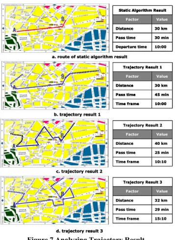
Figure 7 shows static algorithm result route and trajectory results to analyzing the result with ORDF.
A
B
30 min Pass time
10:00 Departure time
30 km Distance
Value Factor
Static Algorithm Result
a. route of static algorithm result A
B
30 min Pass time
10:00 Departure time
30 km Distance
Value Factor
Static Algorithm Result
A
B
30 min Pass time
10:00 Departure time
30 km Distance
Value Factor
Static Algorithm Result
a. route of static algorithm result
A
B
45 min Pass time
10:00 Time frame
30 km Distance
Value Factor
Trajectory Result 1
b. trajectory result 1 A
B
45 min Pass time
10:00 Time frame
30 km Distance
Value Factor
Trajectory Result 1
A
B
45 min Pass time
10:00 Time frame
30 km Distance
Value Factor
Trajectory Result 1
b. trajectory result 1
A
B A
B
25 min Pass time
10:10 Time frame
40 km Distance
Value Factor
Trajectory Result 2
c. trajectory result 2 A
B A
B A
B A
B
25 min Pass time
10:10 Time frame
40 km Distance
Value Factor
Trajectory Result 2
c. trajectory result 2
A
B A
B
29 min Pass time
15:10 Time frame
32 km Distance
Value Factor
Trajectory Result 3
d. trajectory result 3 A
B A
B
29 min Pass time
15:10 Time frame
32 km Distance
Value Factor
Trajectory Result 3
d. trajectory result 3
Figure 7 Analyzing Trajectory Result
We define factor f0 is distance, f1 is pass time, f3 is time frame and allocate weight to each factor, w(f0) = 0.1, w(f1)
= 0.4, w(f2) = 0.5. In this case, we consider f3 time frame as most important factor. The result of Route Cost is Cost(T1 )=1.8, Cost(T1 )=1.7, Cost(T1 )=6.8 in case
defining normalized function as just ordering value simply. In this figure 7, static route and trajectory 1 is same distance and similar time frame but pass time is longer than 30 min in experiential real environment. And generally time frame factor can be important factor because in the similar time frame, the information of route like distance, pass time is more reliable. In this paper, we define normalized function as simply but normalized function must be more complicated in order to enhance reliability, correctness to determine optimal route.
5. FUTURE WORKS
In this paper, just we define logical model to determine optimal route for travelling and some function and logic is defined very simply. But next time we will elaborate this model and implement system to be applicable in real telematics and LBS fields. We have been scheduling to get the large volume of historical location of real vehicles.
So, after implementing system, we will be able to estimate system performance and reliability of result route.
References:
Dieter Pfoser, Christian S. Jensen, and Yannis Theodoridis, "Novel Approaches in Query Processing for Moving Object Trajectories," VLDB 2000, 395-406 E. W. Dijkstra, “A Note on Two Problems in Connection with Graphs”, Number Mathematics, Vol. 1, pp.269 – 271, 1959
Jensen, C. S. Jensen, A. Friis-Christensen, T. B. Pedersen, D. Pfoser, S. Saltenis, and N. Tryfona, “Location-Based Services – A Database Perspective” Proceedings of the Eighth Scandinavian Research Conference on Geographical Information Science, As, Norway, June 25- 27, 2001, pp. 59-68
Ouri Wolfson, Bo Xu, Sam Chamberlain, Liqin Jiang,
"Moving Objects Databases: Issues and Solutions", Proc.
of the 10th Int. Conf. on Scientific and Statistical Database Management (SSDBM98), Capri, Italy, July 1-3, 1998, pp. 111-122
Ralf H. Guting, Mike H. Bohlen, Martin Erwig, Christian S. Jensen, Nikos A. Lorentzos, Markus Schneider, Michalis Vazirgiannis, “ A Foundation for Representing and Querying Moving Objects,” ICDE, pp.422-432, 1997 R. W. Hall, “The Fastest Path through a Network with Random Time-Dependent Travel Times”, Transportation Science Vol. 20, No. 3, pp.182-188
T.Kitamura, M. Kobayashi, K. Takeuchi, “The Dynamic Route Guidance Systems of UTMS”, Proc. Of The Second World Congress on Intelligent Transport Systems 95 YOKOHAMA, pp.610-615, 1995