for Marine Environmental Engineering
Vol. 12, No. 3. pp. 165-172, August 2009165
이중적분을 이용한 완경사면에서의 선형파 방정식
김효섭
†
·정병순·이예원 국민대학교 건설시스템공학부A Linear Wave Equation Over Mild-Sloped Bed from Double Integration
Hyoseob Kim
†
, Byung Soon Jung and Yewon LeeDepartment of Civil and Environmental Engineering, Kookmin University, Seoul, Korea
요 약
연직 2차원 평면을 대상으로 하는 연속방정식을 수심방향으로 이중적분 하여 수평1차원 파랑방정식을 구하였다. 새 방정식은 복소수 포텐셜 함수로 구성되어 있으며, 파랑의 진폭과 위상경사함수를 도입하여 한 세트의 실수방정식으 로도 변형되었다. 파랑진폭과 위상경사함수를 포함한 한 세트의 식은 각각 1차, 2차 상미분방정식이며, 한쪽 경계에 서 경계조건을 적절히 지정하여 전 영역에서의 해를 한 방향으로 진행하면서 구할 수 있다. 이때 경계조건으로는 파 랑진폭 값, 파랑진폭의 경사, 위상 경사 값이다. 단순한 중앙차분식을 이용하여 식을 차분화 하였다. 새 방정식을 Booij의 경사판, Massel의 부드러운 저면, Bragg의 싸인 함수의 저면에 대하여 적용하여 보았다. 본 방정식은 Massel의 수정완경사방정식, Berkhoff 의 완경사방정식, 완전 선형방정식과 비교하여 유사한 결과를 나타내었으며, 유용함을 보였다.
Abstract − A set of equations for description of transformation of harmonic waves is proposed here. Velocity potential function and separation of variables are introduced for the derivation. The continuity equation is in a vertical plane is integrated through the water so that a horizontal one-dimensional wave equation is produced.
The new equation composed of the complex velocity potential function, further be modified into. A set up of equations composed of the wave amplitude and wave phase gradient. The horizontally one-dimensional equations on the wave amplitude and wave phase gradient are the first and second-order ordinary differential equations. They are solved in a one-way marching manner starting from a side where boundary values are supplied, i.e. the wave amplitude, the wave amplitude gradient, and the wave phase gradient. Simple spatially-centered finite difference schemes are adopted for the present set of equations. The equations set is applied to three test cases, Booij’s inclined plane slope profile, Massel’s smooth bed profile, and Bragg’s wavy bed profile. The present equations set is satisfactorily verified against existing theories including Massel’s modified mild-slope equation, Berkhoff’s mild- slope equation, and the full linear equation.
Keywords: Double integral(이중적분), Leibniz rule(Leibniz 법칙), Mild-sloped bed(완경사면), Wave amplitude (파랑진폭), Wave phase gradient(파랑위상의 경사)
1. INTRODUCTION
The mild-slope equation has been widely used for the description of wave transformation over mild-sloped sea beds since it was proposed by Berkhoff [1973]. A sea bed
is often called mild-sloped when the bed slope is much smaller than 1, or smaller than 1/3. The mild-slope equation was developed from either the continuity equation or the principle of stationary action by including the variational principle. It has been known that the accuracy of the mild- slope equation is guaranteed up to a certain bed slope.
Berkhoff [1973] derived the mild-slope equation starting
†
Corresponding author: [email protected]
from the continuity equation. Water was assumed to be incom- pressible and the flow inside free surface waves was assumed to be irrotational, which allowed using velocity potential function, Φ. The continuity of mass flow in the x z domain is expressed by the following Laplace equation:
(1)
where x is the horizontal coordinate, and z is the upward vertical coordinate over the still sea level. The continuity of mass flow should be satisfied at every point in the compu- tational domain at every instant. Likewise, the continuity equa- tion should be satisfied at every section in the computational domain at every instant. The integration of the continuity equation multiplied by an arbitrary weight function at any selected section should also be satisfied at every instant.
Berkhoff chose a hyperbolic cosine function as the weight function in the vertical direction to take into account verti- cal distribution of wave energy flux, and took the vertical integration process of the following equation which is the multiplication of the continuity equation and the vertical weight function, Z of Equation (3):
(2)
and
(3)
Berkhoff additionally made use of Green’s theorem related to the bed boundary condition, obtained the final form of the mild-slope equation. The mild-slope equation has also been proposed in different types of partial differential equation by Rather [1979] and Copeland [1985].
More recently the modified mild-slope equation was pro- posed by Massel [1993], and Chamberlain and Porter [1995].
Two time-dependent forms of the modified mild-slope equation were presented by Suh et al. [1997] by using Green’s theorem, and the variational principle in the manner that Luke [1967]
confirmed the Eulerian equations of motion for the classical water wave problem. Suh et al.’s equations are transformed into Massel’s modified mild-slope equation when the time- dependent term is replaced by a time-invariant term. Suh et al. suggested that the modified mild-slope equation could also be used for random waves if the carrier frequency is introduced. The modified mild-slope equation is reduced to the mild-slope equation when some higher-order terms of
the modified mild-slope equation are turned off.
The modified mild-slope equation is known to have the applicability for a wider range of bed slopes than the mild- slope equation. Furthermore the modified mild-slope equa- tion has produced more accurate reflection coefficients for Bragg’s sinusoidal bed tests than the mild-slope equation due to the additional higher-order terms.
The final form of the governing equation is dependent on the weight function to be multiplied to the continuity equa- tion. The weight function may represent the importance of the fluid divergence property in a water column. Here we adopt a constant weight function instead of at hyperbolic cosine function which was adopted in the mild slope equa- tion, and derive a new from of governing equation in the following sections. The new equations are applied to three topographies for comparison with other theories in the last section.
2. THE NEW WAVE EQUATION
At free surface boundary nonlinear terms of the momen- tum equation are ignored, and the following condition in a linear form is applied:
(4)
where t is time, and g is the acceleration due to gravity, while at the bed the following zero fluid flux condition is applied:
(5)
where h is the water depth relative to the still water level.
Now, we integrate the equation of mass continuity with respect to z from -h to 0.
(6)
Equation (6) is often used to calculate vertical velocities at an arbitrary level when the horizontal velocity field is known. Equation (6) can be thought as the integral of the continuity equation without additional weight function over the water column. It should be noted that the expression with the integration at a section is less strict than the expres- sion with the partial differential equation which is valid at every point in the domain. The above integral with two
∂ 2 Φ
∂ x 2 --- ∂ 2 Φ
∂ z 2 ---
+ = 0
Z ∂
2 Φ
∂ x 2 --- ∂ 2 Φ
∂ z 2 ---
⎝ + ⎠
⎛ ⎞ z d
h –
∫
0 = 0
Z coshk z h ( + ) coshkh ---
=
∂ Φ --- ∂ z g∂
2 Φ
∂ t 2 --- –
=
∂ Φ --- ∂ z dh ---∂ Φ dx
--- ∂ x –
=
∂ 2 Φ
∂ x 2 --- ∂ 2 Φ
∂ z 2 ---
⎝ + ⎠
⎛ ⎞ z d
h –
∫
0 = 0
integrands is split into two integrals for convenient descrip- tion. Expanding the Leibniz rule for a second order differ- ential equation, we obtain for the first term of the above equation:
(7)
=
= (8)
Harmonic waves are of interest in this paper, and variables can be separated as:
(9) where Z is given by Equation (3), the complex function φ is dependent on x, and the complex phase function Ω is dependent on time only as:
(10) where i = , and ω is the wave angular velocity.
Then,
(11)
where λ is the deep water wave number, ω
2
/g. The free sur- face boundary condition, Equation (4), is transformed into the dispersion relationship:(12) Inserting Equations (9) and (10), into Equation (8), we obtain:
(13) where
(14)
and
(15)
Equation (13) can be extended to a three-dimensional form by including the other horizontal coordinate, y, which reads:
(16) where is the gradient vector on the x y plane.
Up to the present the bed boundary condition has not yet been reflected in the governing equation in any way. When Equation (9) including the hyperbolic cosine function of Equa- tion (3) is applied to the bed boundary, the left side of the bed boundary condition, Equation (5), becomes zero, which leads to simple zero horizontal and vertical velocities at the bed. The right side of the bed boundary condition, Equation (5), reads:
(17)
Then, the second derivative of the potential function becomes:
=
= (18)
Replacing the second and first derivatives of the govern- ing equation, Equation (13), by the potential function using Equations (17) and (18), we obtain:
(19) where F is a function of x, k and h. Since Equation (18) should always be satisfied, F=0. This new relationship between x, k and h comes into conflict with the dispersion relationship between k and h derived from the free surface boundary condition. Therefore, we convey this mismatch of the mass conservation at the bed to evanescent modes instead of applying of this bed boundary condition to the hori- zontally propagating mode, although the evanescent modes are not of main interest of this paper. We also see that the mild- slope equation and the modified mild-slope equation and com- plementary mild-slope equation (Kim and Bai’s [2004]),
∂ Φ ∂ x --- z d
h –
∫
0 = dx --- d∫– 0 h Φ z d – Φ dh --- dx – h
∂ 2 Φ
∂ x 2 --- z d
h –
∫
0 dx --- ∂ Φ d
∂ x --- z d
h –
∫
0 – ∂ Φ dh dx ---
∂ x ---
h –
=
d dx --- d
dx --- Φ z d
h –
∫
0 – dh dx ---Φ – h
⎝ ⎠
⎛ ⎞ dh
dx ---∂ Φ
∂ x ---
–
–
=
d 2 dx 2 --- Φ z d
h –
∫
0 2dh ---∂Φ dx --- ∂ x
h –
– d 2 h
dx 2 ---Φ – h
– dh
--- dx
⎝ ⎠ ⎛ ⎞ 2 ∂ Φ --- ∂ z
–
+
=
Φ = exp ( – i ωt )
Ω = exp ( – i ωt ) 1 –
Z z d
h –
∫
0 = k ---- λ 2
λ
--- k = tanhkh
d 2 φ dx 2
--- 2k 4 2kh sinh2kh + --- 1
sinhkh ---
⎝ – ⎠
⎛ ⎞dh
dx ---dΦ --- dx +
+ k 2 2f 1 --- k k
sinhkh ---
⎝ + ⎠
⎛ ⎞d 2 h
dx 2 ---
– 6f 1 2
k 2 --- 2f 2
--- k
– 2k 2 + 2khf 1 coshkh ---
⎝ + ⎠
⎜ ⎟
⎛ ⎞ dh
dx ---
⎝ ⎠ ⎛ ⎞ 3
⎩ + ⎭
⎨ ⎬
⎧ ⎫ φ=0
f 1 dk
dh --- 2k 2 2kh sinh2kh + --- –
= =
f 2 df 1
--- dh 8k 3 2kh sinh2kh +
( ) 3
--- 2kh sinh2kh cosh { + ⋅ ( 2 kh + 1 ) }
= =
∇ 2 Φ 2k 4
2kh sinh2kh + --- 1
sinhkh ---
⎝ – ⎠
⎛ ⎞∇h ∇Φ ⋅
+
+ k 2 2f 1 --- k k
sinhkh ---
⎝ + ⎠
⎛ ⎞∇ 2 h
– 6f 1 2
k 2 --- 2f 2
--- k
– 2k 2 + 2khf 1 coshkh ---
⎝ + ⎠
⎜ ⎟
⎛ ⎞
∇h ( ) 2
⎩ + ⎭
⎨ ⎬
⎧ ⎫ φ=0
∇
d φ
dx --- ( k + hf 1 )tanhkhdh ---φ dx
=
d 2 φ dx 2 --- d
dx --- k hf ( + 1 )tanhkhdh --- dx
⎩ ⎭
⎨ ⎬
⎧ ⎫ φ ( k + hf 1 )tanhkhdh
dx ---
⎩ ⎭
⎨ ⎬
⎧ ⎫dφ
--- dx +
=
d
dx --- k hf ( + 1 )tanhkhdh dx ---
⎩ ⎭
⎨ ⎬
⎧ ⎫ φ ( k + hf 1 )tanhkhdh
dx ---
⎩ ⎭
⎨ ⎬
⎧ ⎫ 2 φ
+
d
dx --- k hf ( + 1 )tanhkhdh dx ---
⎩ ⎭
⎨ ⎬
⎧ ⎫
k + hf 1
( )tanhkhdh
--- dx
⎩ ⎭
⎨ ⎬
⎧ ⎫ 2
+ φ
F x k h ( , , )φ 0 =
require evanescent modes for full agreement at the bed, see Massel [1993]. Trials have been attempted to incorporate the evanescent modes in dealing with the wave propagation problems over sloped beds by some researchers.
Now we arrange the developed equation in a simple form to compare with existing equations. We can compare the new equation with the previous mild-slope equation of Berkhoff and the modified mild-slope equation proposed by Massel or Chamberlain and Porter. The one-dimensional versions of the new equation, mild slope equation and the previous mod- ified mild-slope equation are arranged in the following form:
(20)
We non-dimensionalize the coefficient function A of the modified mild-slope equation by multiplying the water depth as:
Ah = (21)
and that of the developed equation:
(22)
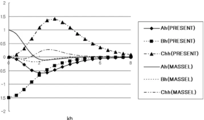
see Fig. 1
The non-dimensional variable group, Ah, of the present equation decreases as the independent variable group, kh, increases up to about 2. After that the Ah increases slowly as kh increases. This trend of variable group Ah of the present equation is similar to the trend of Ah of the mod- ified mild-slope equation. However the starting value of Ah of the present equation is 0 instead of 1 for the mod- ified mild-slope equation.
The non-dimensional variable group, Bh, of Equation (13) monotonously increases as kh increases, while Bh of the modified mild-slope equation decreases as kh increases up to about 2, and then increases slowly as kh increases after that. The starting value of Bh of the present equation is -1.5, which is smaller than the value 0 of the modified mild-slope equation.
The non-dimensional variable group, Ch
2
, of the present equation increases as kh increases up to about 3, and then decreases after that. The variable group Ch2
of the modified mild-slope equation has similar trend to the present equa- tion, but the variation of Ch2
of the present equation is much larger than that of the modified mild-slope equation.We express the developed equation in a simpler form for compact expression as:
(23)
Here we introduce the wave amplitude, a, the wave phase, S, and its spatial gradient, b, as:
(24) The wave amplitude, the wave phase, and its gradient are dependent on x for one-dimensional problems. Then, Equa- tion (23) is split into the following two equations composed of real variables only as:
(25)
and
(26)
Either Equation (23) of a complex variable or a set of Equations (25) and (26) of real variable can be solved for wave transformation over mild-sloped beds.
3. NUMERICAL SOLUTION
We adopt explicit finite difference schemes to solve Equa- tions (25) and (26). First, Equation (25) is discretized as
d 2 φ
dx 2 --- Adh
dx ---dφ
dx --- k 2 B d 2 h dx 2 --- C dh
dx ---
⎝ ⎠ ⎛ ⎞ 2
+ +
⎩ ⎭
⎨ ⎬
⎧ ⎫
φ
+ + = 0
2kh 2kh sinh2kh +
( ) 2
--- 3sinh2kh 2kh 1 2sinh { + ( – 2 kh ) }
Ah 2kh 4
2kh sinh2kh + --- 1
sinhkh ---
⎝ – ⎠
⎛ ⎞
=
d 2 φ dx 2 --- Ddφ
dx --- Eφ
+ + = 0
D A dh --- dx
=
E k 2 B d 2 h dx 2 --- C dh
dx ---
⎝ ⎠ ⎛ ⎞ 2
+ +
=
φ ae = iS
d 2 a dx 2 --- Dda
dx --- ( E b – 2 )a
+ + = 0
db dx --- 2
a ---da dx --- D +
⎝ ⎠
⎛ ⎞b
+ = 0
Fig. 1. Coefficient functions of present and modified mild-slope
equations.
(27)
and Equation (29) is discretized as
(28)
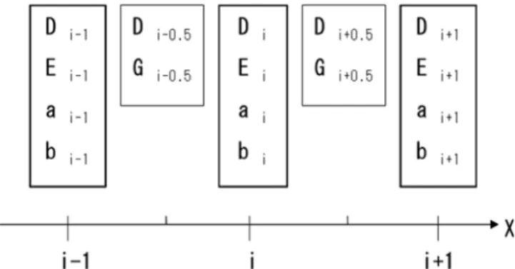
Boundary conditions should be provided to slove the equation. Assume that answers are given at the on-shore boundary where only transmitted waves exist. Therefore, a, da/dx and b at the right end of the computational domain are provided, in other words discrete variables a
M
, aM-1
, bM
are provided to the finite difference equations. The two finite difference equations are alternately solved: Equation (27) is transformed into Equation (21) for a
i-1
, and Equation (28) is transformed into Equation (30) for bi-1
. Both difference equa- tions are centred in space, see Fig. 2:(29)
and
(30)
where
(31)
Equations (29) and (30) are solved in the negative x direction.
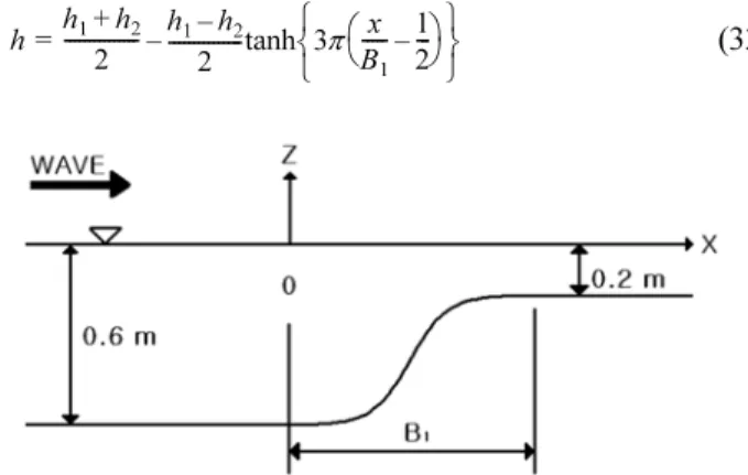
4. VERIFICATION OF NEW EQUATION The new set of equations is applied to a series of bed profiles used by Booij [1983]. The bathymetry is composed of an inclined plane with a variable slope, which connects
the two flat beds at off-shore and near-shore sides. The hor- izontal width of the plane is called B. When the slope becomes infinite, the shape becomes a step, see Fig. 3. The offshore water depth is 0.6 m, the near-shore water depth is 0.2 m, and the wave period of the incident waves is 2 sec.
The boundary values at the right end of the computation domain were provided considering the fact that only outgo- ing waves exist at the near-shore end. The wave amplitude, a, at the near-shore boundary was given 0.1 m, and the value of the phase function derivative, b, was given the wave num- ber at the shallow zone. The two dependent variables, a and b, were alternately computed from Equations (29) and (30) from the near-shore to the off-shore end.
Computed spatial distribution of the relative wave ampli- tude to the outgoing wave amplitude, a
0
, for a specific plane inclination, width, i.e. B=2 m, 0≤ x ≤ 2 m is shown in Fig. 4.The wave amplitude shows undulation at off-shore side from the inclined plane because of the superposition of the inci- dent and reflected waves.
The computed spatial distribution of the wave phase gra- dient function for a specific plane inclination width of 2 m, 0≤ x ≤ 2 m is shown in Fig. 5. The wave phase gradient function also has undulation at off-shore side from the inclined
a i 1 – – 2a i + a i 1 +
Δx 2
--- D i a i 1 + – a i 1 –
--- Δx ( E i – b i 2 )a i
+ + = 0
b i – b i 1 –
--- Δx 4 a ( i – a i 1 – ) Δx a ( i + a i 1 – ) --- D + i 0.5 –
⎩ ⎭
⎨ ⎬
⎧ ⎫b i + b i 1 –
--- 2
+ = 0
a i 1 – 1 2 D – i Δx
--- 4 2 E [ { – ( i – b i 2 )Δx 2 }a i – ( 2 D + i Δx )a i 1 + ]
=
b i 1 – 2 G + i 0.5 – 2 G – i 0.5 – ---b i
=
G i 0.5 – 4 a ( i – a i 1 – ) Δx a ( i + a i 1 – ) --- D + i 0.5 –
=
Fig. 2. Variable numbering system in finite difference equations set. Fig. 3. Booij’s test step with inclined plane.
Fig. 4. Computed spatial distribution of relative amplitude for
Booij’s bed profile of B=2 m.
plane because of the superposition of incident and reflected waves in the region.
The reflection coefficient, K
r
, can be obtained from the computed maximum and minimum wave amplitudes, amax
and amin
, at the off-shore flat bed zone, that is:(32)
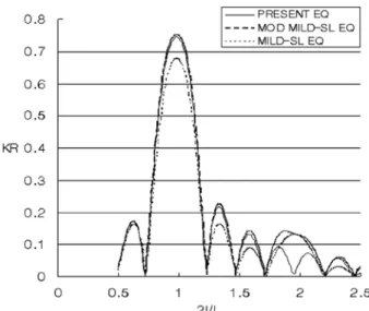
The computed reflection coefficients from the present equa- tion for Booij’s test profiles are shown in Fig. 3. In general the reflection coefficients of the present equation are close to those of the modified mild-slope equation. The reflection coefficients of the present equation are slightly smaller than those of the modified mild-slope equation for inclined plane of slope between 0.4 and 4. It is inferred that the differ- ences come from the different weight functions involved in the integration.
The computed results of the present set of equations were also compared with the solutions of the full linear equation which does not involve separation of variables in Fig. 3 (Park et al. [1991]). The computed reflection coefficients
from the developed equation are closer to the full linear equation solutions than those from the modified mild-slope equation in a range of B smaller than 0.4 m. The reflection coefficients from the present equation, the modified mild- slope equation, and the full linear equation are very close for B larger than or equal to 1 m, because the higher order terms become negligible when the bed slope is small.
For the plane slopes of greater than or equal to 1, which correspond to B≤0.4 m, the computed reflection coefficients from the developed set of equations and the modified mild- slope equation show quite large gaps compared to those from the full linear equation. It has been known that the slope of 1 is the limit slope to the applicability of the mild- slope equations group (Porter and Staziker, [1995]).
The reflection coefficients from the mild-slope equation are quite smaller than those from the developed equations and the modified mild-slope equation in a wide range of bed slopes, especially for steep slopes. The difference may come from the existence of the higher-order terms of the devel- oped equations, or the modified mild-slope equation.
Suh et al. [1997] examined the role of the two higher- order terms, the second derivative of the bed slope and the square of the first derivative of the bed slope, in the mod- ified mild-slope equation on the reflection coefficient for Booij’s bathymetry, and suggested that the discontinuity of bed slope may cause inaccurate reflection coefficient for steep slopes. Tests on bathymetry with no slope discontinu- ity will be useful to look in the cause of the inaccuracy for steep bed slopes.
The developed equation was applied to a set of different bed geometries to examine the effect of the discontinuity of the bed slope on the reflection coefficient. We use Massel’s [1993] bathymetry profile to test the present equation, which is described by:
(33)
K r a max – a min
a max + a min ---
=
h h 1 + h 2 --- 2 h 1 – h 2
---tanh 3π 2 x B 1 --- 1
2 ---
⎝ – ⎠
⎛ ⎞
⎩ ⎭
⎨ ⎬
⎧ ⎫
–
=
Fig. 6. Comparison of computed reflection coefficients for Booij’s
bed profile. Fig. 7. Massel’s smooth bathymetry with hyperbolic tangent funtion.
Fig. 5. Computed spatial distribution of phase gradient for Booij’s
bed profile of B=2 m.
where h is the water depth of the profile, h
1
is the off-shore constant water depth, h2
is the near-shore constant water depth, and B1
is the width of region with non-plane bottom profile. The same off-shore and near-shore water depths as Booij’s bed profiles are chosen to separate out the effect of the discontinuity of the bed slope so that we can compare the test results of the present equation for smooth profiles with the test results for Booij’s test profiles, i.e. h1
=0.6 m, and h2
=0.2 m. For comparison in a figure, Massel’s smooth step results are represented by the steepest slope in the whole profile, 1.5π(h1
-h2
)/B1
, and its corresponding conceptual bottom width, B=B1
/1.5π. The computed reflection coefficients (Kr
) for Massel’s profiles are shown in Fig. 8 with those for Booij’s bed profiles. The computation results show that the reflection coefficient decreases monotonously as the slope becomes milder in contrast to the wave-length-related peri- odic pulses of the reflection coefficient for Booij’s test steps.The reflection coefficient for a uniform slope of Booij’s step is larger than that for the same representative maxi- mum slope of Massel’s smooth step. However, the reflec- tion coefficients for the angled and smooth profiles are not much different for steep slopes even though the slopes are represented by the maximum slopes for the smooth profiles.
The test results of the present equation show that the reflec- tion coefficient increases as the bed slope increases for smooth profiles as well as inclined plane profiles. This indi- cates that there is a limiting bottom slope on the applicabil- ity of the present equation like the modified mild-slope equation maybe because of the adoption of the separation of variables in the velocity potential function.
The present equation is then applied to Bragg’s bathym- etry to examine the accuracy of the developed equation. It has been known that sinusoidal bathymetry can cause high reflection depending on the ratio between the bed form length
and the wave length. The bathymetry is expressed by the following equation:
, x < 0
, 4l > x (34)
where h is the water depth in m, h
1
and h2
are the off-shore and near-shore water depths from the bed forms, respec- tively, and l is the ripple length. Incident waves propagate in the positive x direction. Calling the wave length L, the computed reflection coefficient for 2l/L=0.98 from the present equation is 0.745, which closely agrees with 0.752 from the modified mild-slope equation, while the reflection coefficient of 0.678 from the mild-slope equation is quite smaller than the other results.An interesting feature is the distribution of the reflection coefficient around the second resonance point, i.e. 2l/L=2.
The compared equations produce different distribution of
h 1 = 0.156
h = h 1 – 0.05sin 2πx l⁄ ( ) 0 x 4l ≤ ≤ h 2 = 0.156
Fig. 8. Comparison of computed reflection coefficients for Massel’s smooth bed profiles.
Fig. 9. Bragg’s sinusoidal bathymetry with 4 ripples.
Fig. 10. Comparison of computed reflection coefficients for Bragg’s
bed profile.
the reflection coefficients around the point. The present set of equations produces a mode, other equations produce more or less high secondary reflection coefficient around 2l/L=2, see Fig. 10. Further study is needed for the explanation of the reason for the differences.
5. CONCLUSIONS
An equation on a complex velocity potential function form for description of the transformation of harmonic waves has been proposed in the present paper. The continuity equation was multiplied by a vertically constant weight function instead of the hyperbolic cosine function which was used to derive the previous mild-slope equation, and the vertical integration process was carried out to the equation. The developed governing equation on the complex velocity potential func- tion was also expressed in a set of two equations composed of the wave amplitude and phase gradient function.
The present set of equations was applied to the three bed profiles, Booij’s inclined bed profile, Massel’s smooth bed profile, and Bragg’s wavy ripple bed profile. The equations set was verified against other theories.
The test of the present equations set on Booij’s steps reveals that the present equation provides accurate reflection coef- ficient compared to the solutions from the full linear equa- tion. The present equation behaves similarly to the modified mild-slope equation, but shows slightly more accurate reflec- tion coefficient than the modified mild-slope equation for relatively steep bottom slopes. The test of the present equa- tions set on Massel’s smooth steps exhibits that the reflec- tion coefficient increases as the bed slope increases even though the bed slope changes continuously throughout the bed profile. The test of the present equations set on Bragg’s sinusoidal ripples confirms that the present equations set produces correct reflection coefficient to the modified mild- slope equation, over a wide rage of ratio between the ripple length and the wave length.
The three sets of experiments confirm the accuracy and applicability of the new equation based on the vertically uni- form weight function.
ACKNOWLEDGEMENTS
The work was supported by Korean Ministry of Land, Transport and Maritime Affairs, and Korea Institute of Marine Science & Technology Promotion under the title of “Marine and Environmental Prediction System (MEPS)” in 2009, and by Kookmin University as a university grant in 2009.
REFERENCES