Nonparametric Bayesian Multiple Comparisons for Geometric Populations

2005, Vol. 16, No. 4, pp. 1129∼1140

Nonparametric Bayesian Multiple Comparisons for Geometric Populations

M. Masoom Ali¹⁾ ⋅ Cho, J.S²⁾ ⋅ Munni Begum³⁾

Abstract

A nonparametric Bayesian method for calculating posterior probabilities of the multiple comparison problem on the parameters of several Geometric populations is presented. Bayesian multiple comparisons under two different prior/ likelihood combinations was studied by Gopalan and Berry(1998) using Dirichlet process priors. In this paper, we followed the same approach to calculate posterior probabilities for various hypotheses in a statistical experiment with a partition on the parameter space induced by equality and inequality relationships on the parameters of several geometric populations. This also leads to a simple method for obtaining pairwise comparisons of probability of successes. Gibbs sampling technique was used to evaluate the posterior probabilities of all possible hypotheses that are analytically intractable. A numerical example is given to illustrate the procedure.

Keywords : Dirichlet Process Prior, Geometric Distribution, Gibbs Sampler, Mixture of Dirichlet Processes, Multiple Comparison, Nonparametric Bayes

1. INTRODUCTION

The geometric model has been widely used as a model in areas ranging from studies on the inspection of defective items to research involving statistical quality control. We consider the multiple comparisons problem (MCP) for K geometric populations with parameters θ = (θ_{1, ,}θ_K), the probabilities of successes, to make

1) First Author : Department of Mathematical Sciences, Ball State University, Muncie, IN 47306-0490, U.S.A.

2) Department of Informational Statistics, Kyungsung University, Pusan, Korea, 608-736 3) Department of Mathematical Sciences, Ball State University, Muncie, IN 47306-0490,

U.S.A.

inferences on the relationships among the θ_i's based on observations. With equality and inequality relationships among θ_i's we can set up statistical hypotheses as under,

H₀: θ₁= θ₂= = θ_K,

H₁: θ₁≠ θ₂, θ₂= θ₃= = θ_K,

H_N: θ₁≠ θ₂≠ θ₃≠ ≠ θ_K. (1)

To our knowledge, the multiple comparison problem (MCP) among K geometric populations has not been studied yet, partly because of the difficulty in handling the distributional aspects and the computations. The Bayesian approach to the MCP for beta/bionomial and normal/inverted gamma studied by Gopalan and Berry(1998), is extended here to the geometric populations. In a Bayesian MCP problem, prior probabilities on the hypotheses are elicited through specification of a process prior on the parameters of interest θ = (θ_1, , θ_K). Then posterior probabilities are calculated from the posterior distributions induced by the hypotheses. The Dirichlet process prior (DPP) is a typical objective prior specification. The DPP is a prior distribution on the family of distributions, which is dense in the space of distribution functions.

The family of DPPs is introduced by Ferguson(1973) and is extended to mixtures of DPP by Antoniak(1974). The introduction of Markov chain Monte Carlo (MCMC) methods in nonparametric Bayesian modeling was begun with Escobar (1988). Innovations in computations and the development of new MCMC schemes are found in the key contributions by Doss (1994), Bush and MacEachern (1996), Escobar and West (1997), MacEachern and Müller (1998), West, Müller and Escobar (1994). Gopalan and Berry(1998) proposed Bayesian multiple comparisons using Dirichlet process priors for applied normal and binomial data.

In this paper, we consider the Bayesian approach to resolve the multiple comparisons problem for the probabilities of successes among K geometric populations, based on an hierarchical nonparametric family of Dirichlet process priors. Calculating posterior probabilities for the hypotheses is analytically intractable but can easily be evaluated using Gibbs sampling. In section 2 some reviews on the DPP are given, while section 3 presents the calculation of posterior probabilities for the hypotheses in MCP. A numerical example illustrating the procedure is described in section 4.

2. PRELIMINARIES

The Dirichlet process prior G is determined by two parameters: a distribution function G₀( ) and a positive scalar precision parameter α. G₀( ) defines the location of the DPP. So G₀( ) is sometimes called prior ``guess" or baseline prior. The precision parameter α determines the concentration of the prior for G around the prior guess G₀, and therefore measures the strength of belief in G_0. Then the DPP is denoted as G∼ D(G│G₀, α ). For large values of α, a sampled G is very likely to be close to G₀. For small values of α, a sampled G is likely to put most of its probability mass on just a few atoms.

Mixture of Dirichlet Process models have become increasingly popular for modeling when conventional parametric models would impose unreasonably stiff constraints on the distributional assumptions(such as finite mixture of distributions). Despite of the large variety of applications, the core of the mixture of Dirichlet process model can basically be thought of as a simple Bayes model given by the likelihood and prior with added uncertainty about the prior distribution G∼ D(G│G0,α ). The more complex models typically require another portion to the hierarchy that allows the introduction of distributions on the hyperparameters α and G_0.

Consider K geometric populations with the probabilities of success θ = (θ₁, θ_2, , θ_K). Observations Y= (Y₁, Y₂, , Y_K) are available on these populations, where Y_i= (y_i1, , y_in

i) is n_i 1 vector of conditionally independent observations on population i, i = 1, 2, , K; j = 1, 2, , n_i and

Σ

i = 1 K

n_i= n. Then the probability density function of y_ij is

f (y_ij│θ_i) = θ_i (1− θ_i)^yij, y_ij= 0, 1, 2, . (2) We assume that the θ_i's come from G, and that G∼ D(G│G0, α ). This structure results in a posterior distribution which is a mixture of Dirichlet processes (Antoniak 1974). Using the Polya urn representation of the Dirichlet process (Blackwell and MacQueen 1973), the joint posterior distribution has the form

θ_i∣ Y ∝ ∏^K

i = 1f( y_i∣θ_i)

αG₀(θ_i) +∑

k < iδ(θ_i∣θ_k)

α + i - 1 , (3) where (θ_i│θ_k) is the distribution which has a point mass on θ_k. For each i = 1, , K, the conditional posterior distribution of θ_i is given by

θ_i│θk,k≠ i, Y ∝ q0G_b(θ_i│yi) +

Σ

k≠ i

q_k (θ_i│θk), (4)

where G_b(θ_i│bfyi) is the baseline posterior distribution, q₀∝α

:

f (bfy_i│θi)dG₀(θ_i), q_k∝f (yi│θk) and 1 = q₀+ _k

Σ

The multiple comparison problem of K geometric populations is to make inferences concerning relationships among the θ's based on Y. Let Θ = θ = ( θ_1,θ_2,…,θ_K) : θ_i R, i = 1, 2, , K be the K-dimensional parameter space. Equality and inequality relationships among the θ's induce statistical hypotheses that are subsets of Θ, i.e.,, H₀: θ₀= θ_i: θ₁= θ₂= = θ_K, H₁: θ₁= θ_i: θ₁≠ θ₂= = θ_K and so on up to H_N: θ_N= θ_i: θ₁≠ θ_2≠ ≠ θ_K. The hypotheses H_r: θ_r,r = 0, 1, 2, , N, are disjoint, and ∪^Nr = 0θ_{r =}Θ .

The elements of Θ themselves behave as described by (3) and so with positive probability, they will reduce to some p≤K distinct values. We denote the distinct values of the parameters by putting a superscript * on them. Then any realization of K parameters θ_i generated from G lies in a set of p≤K distinct values, denoted by θ^*= (θ^{* ,}₁θ^{* ,}₂ , θ^*_p). The Gibbs sampling for MCP problem can be described through what is termed as Configuration by Gopalan and Berry (1998).

Their definition of Configuration is restated here,

Definition: The configuration S = S_1,S_{2, ,}S_l determines a classification of θ into p distinct groups or clusters; n_j^θ = number of θ_i's in group j that share the common parameter value θ^*_j. Write K_j for the set of indices of parameters in group j, K_j= i : S_i= j_{. Let} X_j=^X_j: S_i= j^€ be the corresponding group of

n_K

j= _i

Σ

j

n_i observations

There is a one-to-one correspondence between hypotheses and configurations.

And the required computations are reduced by the fact that the distinct θ_i's are typically reduced to fewer than K due to the clustering of the θ_i's inherent in the Dirichlet process. Hence, (4) can be rewritten as:

θ_i│θk,k≠ i, y ∝ q0G_b(θ_i│yi) + _{k = 1}

Σ

*

n_kq_k^* (θ_i│θ^*k), (5)

with q_k^*∝f (y_i│θ^*_k), and 1 = q₀+

Σ

θ_i│G ∼ G (θ_i), (7)

G│G_0,α∼ D(G│G_0,α ), (8)

G₀│ (αoi, _oi)∼ B(αoi, _oi). (9) Here, Ge indicates geometric distribution. Now the choice of the precision parameter α in Dirichlet process is extremely important for the model. Here, we consider the gamma prior for α with a shape parameter a and scale parameter b, that is, α∼ Γ (a, b ). Then the Γ (a, b ) is to be the reference prior by a→0 and b→0. And we have access to a neat data augmentation device for sampling α by Escobar and West(1995).

The configuration notation is more convenient to use in describing the Gibbs sampling algorithm. This results in sampling from the following conditional posterior distributions:

(θ_i│Y, θk, k≠ i, α, αoi, _oi)∼ q0B (n_i+ α_io,

Σ

n_i

y_ij+ _oi)

+ _k

Σ

(10)

(θ^*_j│Y, S, αoi, _oi)∼ B(_k

Σ

j

n_k+ α^*_oj,_k

Σ

j

Σ

ni

y_kl+ ^*_oj), (11) (α│η, K^*)∼π_ηΓ (a + K^*, b− log (η))

+ (1− π_η)Γ (a + K^{*− 1}, b− log (η)),

(12) (η│α, K^{* )}∼ B (α + 1, K ). (13) where

q₀ ∝ α Γ (α_oi+ _oi) Γ (α_oi) Γ ( _oi)

Γ (n_i+ α_oi) Γ (

Σ

n_i

y_ij+ _oi)

Γ (n_i+

Σ

ni

y_ij+ α_oi+ _oi) ,

q_k ∝ θⁿ_kⁱ(1− θ_k)

Σ

yij

.

Gibbs sampling proceeds by simply iterating through (10) - (13) in order, sampling at each stage based on current values of all the conditioning variables.

The configuration gives the equality and inequality relationships among the θ's, which correspond to the partitions on the parameter space Θ and in turn to the hypotheses of interest. To estimate the posterior probability of a hypothesis H_r from a large number(L) of sample draws, we use

P (H_r│Y) 1

L

Σ

where _S

l(H_r) denotes unit point mass for the case where lth draw of S, that is, S_l corresponds to H_r.

The probability of equality for any two θ's can be calculated from the posterior distributions on hypotheses, P (H_r│Y), r = 1, 2, , N. This can be achieved by adding probabilities of those hypotheses in which θ_i and θ_j are equal. For example,

P (θ_i= θ_j│Y) 1 L

Σ

l = 1 L

S_l(θ_i= θ_j) =

Σ

r = 1 N

P (H_r│Y) H_r(θ_i= θ_j), i≠ j, (15)

where _S

l(θi= θj) and _H

r(θi= θj) denote unit point mass for the case where S_l and H_r indicate θ_i= θ_j, respectively.

4. ILLUSTRATIVE EXAMPLE

In this section, we use hypothetical data to illustrate the multiple comparisons for the parameters of geometric populations. Here, we consider 4 geometric populations and sample size of 50 from each geometric distributions. In this paper, we consider multiple comparisons for two cases, so that true hypothesis are H_true: θ₁= θ₂= θ₃≠ θ4 for case I and H_true: θ₁= θ₂≠ θ3= θ₄ for case II, respectively.

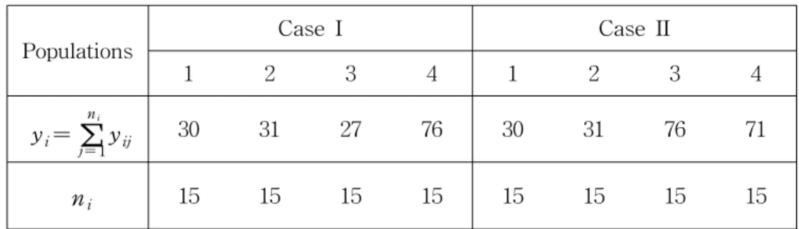
Table 1 The observed summary statistics for each populations

Populations

Case I Case II

1 2 3 4 1 2 3 4

y_i=∑

ni

j= 1y_ij 30 31 27 76 30 31 76 71

n_i 15 15 15 15 15 15 15 15

The observed summary statistics for each case are given as Table 1. And the numbers of possible hypothesis are 15 for each case. For the precision parameter α, we consider three Gamma priors with parameters (a, b )=(1.0, 1.0), (0.1, 0.1) and (0.01, 0.01 ) such that same means 1 and different variances 1, 10, and 100, respectively. Then latter prior is fairly noninformative, giving reasonable mass to both high and low values of α. But, the Γ (1.0, 1.0 ) prior favors relatively low values of α. Also we set that each θ_i,i = 1, , 4 follows in priori beta with parameter α_oi= _oi= 1.0 to reflect vagueness of the prior knowledge. All the calculated posterior probabilities for all possible hypotheses are approximated by the Gibbs sampling algorithm using 40,000 iterations with 20,000 burn-in iterations.

Table 2 and Table 3 give the calculated posterior probabilities for all possible hypotheses of case I and case II, respectively.

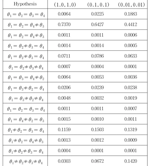
Table 2 Calculated posterior probabilities for each hypothesis with three cases of (a, b ) in Case I

Hypothesis ( 1.0, 1.0) ( 0.1, 0.1) ( 0.01, 0.01)

θ₁= θ₂= θ₃= θ₄ 0.0064 0.0225 0.1883

θ₁= θ₂= θ₄≠θ₃ 0.7370 0.6427 0.4412

θ₁= θ₂= θ₄≠θ₃ 0.0011 0.0011 0.0006

θ₁= θ₂≠θ₃= θ₄ 0.0014 0.0014 0.0005

θ₁= θ₂≠θ₃= θ₄ 0.0711 0.0786 0.0633

θ₁= θ₂≠θ₃≠θ₄ 0.0007 0.0004 0.0001

θ₁= θ₃= θ₄≠θ₂ 0.0064 0.0053 0.0036

θ₁= θ₃≠θ₂= θ₄ 0.0206 0.0239 0.0238

θ₁= θ₃≠θ₂≠θ₄ 0.0048 0.0032 0.0019

θ₁= θ₂= θ₃= θ₄ 0.0011 0.0011 0.0007

θ₁= θ₄≠θ₂= θ₃ 0.0015 0.0010 0.0011

θ₁≠θ₂= θ₃= θ₄ 0.1159 0.1503 0.1319

θ₁≠θ₂= θ₄≠θ₃ 0.0013 0.0012 0.0009

θ₁≠θ₂≠θ₃= θ₄ 0.0004 0.0001 0.0001

θ₁≠θ₂≠θ₃≠θ₄ 0.0303 0.0672 0.1420

It is evident from Table 2, that the hypotheses for "θ₁= θ₂= θ₃≠ θ4" have the largest posterior probabilities 0.7370, 0.6427, and 0.4412 for all priors of the precision parameter α, respectively. This suggests that the data lend greatest support to equalities for θ₁= θ₂= θ₃ and θ₄ being different from the others. Thus this example shows good performance of the Bayesian multiple comparisons method for several geometric parameters.

Table 3 Calculated posterior probabilities for each hypothesis with three cases of (a, b ) in Case II

Hypothesis ( 1.0, 1.0) ( 0.1, 0.1) ( 0.01, 0.01)

θ₁= θ₂= θ₃= θ₄ 0.0079 0.0470 0.2795

θ₁= θ₂= θ₄≠θ₃ 0.0006 0.0010 0.0004

θ₁= θ₂= θ₄≠θ₃ 0.0000 0.0000 0.0000

θ₁= θ₂≠θ₃= θ₄ 0.6763 0.5672 0.3444

θ₁= θ₂≠θ₃= θ₄ 0.1177 0.1192 0.0914

θ₁= θ₂≠θ₃≠θ₄ 0.0072 0.0050 0.0038

θ₁= θ₃= θ₄≠θ₂ 0.0000 0.0000 0.0000

θ₁= θ₃≠θ₂= θ₄ 0.0008 0.0011 0.0009

θ₁= θ₃≠θ₂≠θ₄ 0.0000 0.0000 0.0000

θ₁= θ₂= θ₃= θ₄ 0.0001 0.0002 0.0002

θ₁= θ₄≠θ₂= θ₃ 0.0118 0.0095 0.0071

θ₁≠θ₂= θ₃= θ₄ 0.0016 0.0015 0.0009

θ₁≠θ₂= θ₄≠θ₃ 0.0001 0.0001 0.0002

θ₁≠θ₂≠θ₃= θ₄ 0.1391 0.1487 0.1103

θ₁≠θ₂≠θ₃≠θ₄ 0.0368 0.0995 0.1609

Table 3 indicates that the hypotheses for "θ₁= θ₂≠ θ3= θ₄" have the largest posterior probabilities 0.6763, 0.5672, and 0.3444 for all priors of the precision parameter α, respectively. This suggests that the data lend greatest support to equalities for θ₁= θ₂ and θ₃= θ₄ being different from the others. Also, Thus this example shows good performance of the Bayesian multiple comparisons method for several geometric parameters.

Table 4 Pairwise Posterior Probabilities with three cases of (a, b ) in Case I Hypothesis (1.0, 1.0 ) (0.1, 0.1 ) (0.01, 0.01 )

θ₁= θ_{2 0.8170} 0.7463 0.6939

θ₁= θ_{3 0.7711} 0.6948 0.6570

θ₁= θ_{4 0.0141} 0.0283 0.1916

θ₂= θ_{3 0.8656} 0.8197 0.7644

θ₂= θ_{4 0.0167} 0.0311 0.1945

θ₃= θ_{4 0.0104} 0.0254 0.1901

Table 4 shows the pairwise posterior probabilities for the equalities of pairs of θ 's in case I. By table 4, the equalities of (θ₁= θ₂) and (θ₂= θ₃) have the largest posterior probabilities (0.8170, 0.7463, 0.6939) and (0.8656, 0.8197, 0.7644) for three cases of (a, b ), respectively. This suggests that there is strong evidence in the equalities θ₁= θ₂ and θ₂= θ₃.

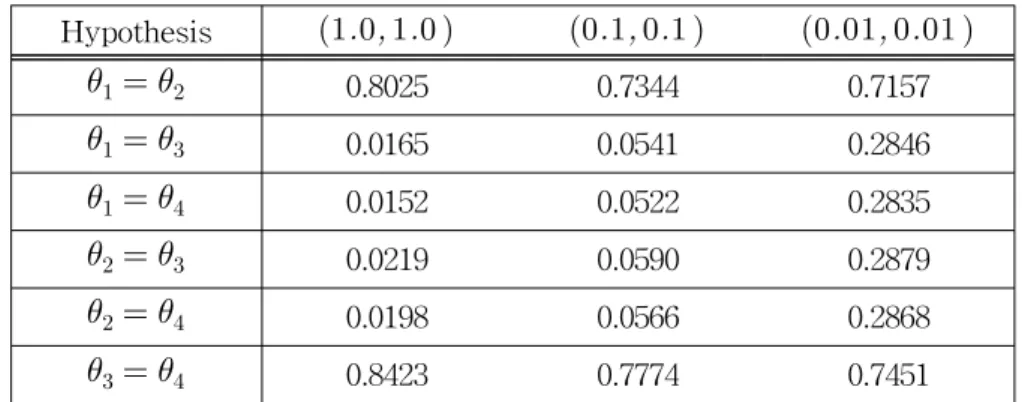
Table 5 Pairwise Posterior Probabilities with threee cases of (a, b ) in Case II Hypothesis (1.0, 1.0 ) (0.1, 0.1 ) (0.01, 0.01 )

θ₁= θ_{2 0.8025} 0.7344 0.7157

θ₁= θ_{3 0.0165} 0.0541 0.2846

θ₁= θ_{4 0.0152} 0.0522 0.2835

θ₂= θ_{3 0.0219} 0.0590 0.2879

θ₂= θ_{4 0.0198} 0.0566 0.2868

θ₃= θ_{4 0.8423} 0.7774 0.7451

Table 5 demonstrates the pairwise posterior probabilities for equality of pairs of θ's in case II. By table 5, the equalities of (θ₁= θ₂) and (θ₃= θ₄) are most large posterior probability (0.8025, 0.7344, 0.7157) and (0.8423, 0.7774, 0.7451) for three cases of (a, b ), respectively. This suggests that there is strong evidence in the equalities θ₁= θ₂ and θ₃= θ₄.

Up to this point, we have considered the problem of developing a Bayesian multiple comparisons for means of K geometric populations. As an alternative to a formal Bayesian analysis of a mixture model that usually leads to intractable

calculations, the DPP is used to provide a nonparametric Bayesian method for obtaining posterior probabilities for various hypotheses of equality among population means.

Extension of the above approach to the multiple comparison problems for the another population is straightforward. The research topics pertaining to the extension of the method and the examination of its performance are worthy to study and are left as a future subject of research.

Acknowledgement : The authors are thankful to the two referees for their careful reading of the manuscript and for their helpful comments.

REFERENCES

1. Antoniak, C.E. (1974), Mixtures of Dirichlet Processes with Applications to Nonparametric Problems, The Annals of Statistics, 2, 1152-1174.

2. Blackwell, D. and MacQueen, J.B. (1973), Ferguson Distribution via Polya Urn Schemes, The Annals of Statistics, 1, 353-355.

3. Bush, C.A. and MacEachern, S.N. (1996), A Semi-parametric Bayesian Model for randomized Block Designs, Biometrika, 83, 275-285.

4. Doss, H. (1994), Bayesian Nonparametric Estimation for Incomplete Data via Successive Substitution Sampling, The Annals of Statistics, 22, 1763-1786.

5. Escobar, M. D. (1988), Estimating the Means of Several Normal Populations by Nonparametric Estimation of the Distribution of the Means. Unpublished dissertation, Yale University.

6. Escobar, M. D. and West, M. (1995), Bayesian Density Estimation and Inference using Mixtures, Journal of the American Statistical

Association, 90, 577-588.

7. Escobar, M. D. and West, M. (1997), Computing Nonparametric Hierarchical Models, ISDS Discussion Paper \#97-15, Duke University.

8. Ferguson, T.S. (1973), A Bayesian Analysis of Some Nonparametric Problems, The Annals of Statistics, 1, 209-230.

9. Gopalan, R. and Berry, D.A. (1998), Bayesian Multiple Comparisons Using Dirichlet Process Priors, Journal of the American Statistical Association, 90, 1130 - 1139.

10. MacEachern, S.N. and Müller, P. (1998), Estimating Mixture of Dirichlet Process Models, Journal of Computational and Graphical Statistics, 7, 223-239.

11. West, M., Müller, P. and Escobar, M.D. (1994), Hierarchical Priors and Mixture Models, with Application in Regression and Density

Estimation, Aspects of Uncertainty : A Tribute to D. V. Lindley (eds:

A.F.M. Smith and P.R. Freeman), London : John Wiley and Sons, 363-386.

[ received date : Sep. 2005, accepted date : Nov. 2005 ]