논문 2016-53-4-13
접지 그리드 설계를 위한 전기 저항 단층촬영법에 기반한 지표의 3차원 저항률 분포 추정
( Three-Dimensional Subsurface Resistivity Profile using Electrical Resistance Tomography for Designing Grounding Grid )
캄밤파티 아닐 쿠마*, 김 경 연**
( Anil Kumar Khambampati and Kyung Youn Kimⓒ)
요 약
대지의 접지 시스템 설치는 안전성과 전기 기기의 올바른 작동을 위해 필수적이며, 대지 파라미터, 특히 토양의 저항률은 대지 접지 시스템 설계에서 결정되어야 한다. 토양의 저항률을 측정하기 위한 가장 흔한 방법은 Wenner의 4전극 방법이 있으 며, 이 방법은 1차원의 저항률을 얻기 위하여 가변 전극 간격을 갖는 큰 측정 세트가 요구되어 번거롭고, 시간소모가 많으며 비용이 많이 든다. 전기 저항 단층촬영법은 저비용이며 빠른 측정이 가능하다는 장점 때문에 토양의 저항률 분포를 추정하기 위해 적용될 수 있다. 전기 저항 단층은 관심지역에 놓인 전극에서 얻은 측정데이터를 사용하여 토양 저항률 분포를 특성화한 다. 이때 전기 단층 촬영법의 역문제는 비선형성이 강하여 저항률 분포를 추정하기 위하여 Tikhonov 조정 방법을 갖는 반복적 Gauss-Newton 방법을 사용한다. 다양한 시뮬레이션을 수행하여 3차원 토양의 저항률 분포를 추정하는데 전기 저항 단층 촬 영법은 유용한 성능을 제공하고 있음을 확인하였다.
Abstract
Installation of earth grounding system is essential to ensure personnel safety and correct operation of electrical equipment. Earth parameters, especially, soil resistivity has to be determined in designing an efficient earth grounding system. The most common applied technique to measure soil resistance is Wenner four-point method. Implementation of this method is expensive, time consuming and cumbersome as large set of measurements with variable electrode spacing are required to obtain a one dimensional resistivity plot. It is advantageous to have a method which is of low cost and provides fast measurements. In this perspective, electrical resistance tomography (ERT) is applied to estimate subsurface resistivity profile. Electrical resistance tomograms characterize the soil resistivity distribution based on the measurements from electrodes placed in the region of interest. The nonlinear ill-posed inverse problem is solved using iterated Gauss-Newton method with Tikhonov regularization. Through extensive numerical simulations, it is found that ERT offers promising performance in estimating the three-dimensional soil resistivity distribution.
Keywords: Electrical resistance tomography, Soil resistivity, Four-point method, Inverse problem, Imaging
*정회원, 제주대학교 원자력과학기술연구소
(Institute for Nuclear Science and Technology, Jeju National University)
**정회원, 제주대학교 전기전자통신컴퓨터공학부 전자
공학전공
(Department of Electronic Engineering, Jeju National University)
ⓒCorresponding Author(E-mail: kyungyk@jejunu.ac.kr)
※ This research was supported by the 2015 scientific promotion program funded by Jeju National University.
Received ; March 15, 2016 Revised ; April 1, 2016 Accepted ; April 6, 2016
Ⅰ. Introduction
Electronic equipment has become an integral part of our everyday lives. Due to technological advancements, these equipment operate at low voltages hence are more sensitive to hazards created due to poor grounding. An efficient grounding system ensures the operation of sensitive equipment from hazards of transients, harmonics and lightning strike and also provides personal safety[1~2]. Surveying of construction site is necessary for installing a proper
grounding system. A conductor or group of conductors which connect the equipment to earth is called the ground electrode. When the object is grounded it is forced to assume the same potential as earth. If the grounded object has different potential to earth then the electric current will pass through the system until the potential difference between the two becomes zero. Grounding systems are designed to control the potential differences in and around the equipment setup. A grounding system constitutes ground conductors, ground rods, equipment to be grounded and the earth itself. Earth model and its parameters have to be determined for designing grounding grid. Earth structure is usually complex and the resistivity of soil and rock varies with region and depth. This variation poses a great challenge in designing the earth grounding system. The earth resistance primarily depends on soil resistivity which in turn depends on factors like soil type, chemical composition, grain size, seasonal variation with respect to temperature etc.
Several methods have been discussed in literature for measuring earth resistance. Most accurate method for measuring a large volume of undisturbed earth is the four-point method. Wenner and Schullemburger methods are the popular of the four-point methods[3~5]. Using four-point method, several sets of arrays of different spacing are required to obtain a one-dimensional plot of resistivity. A large number of measurements are required for surveying the entire construction plot, which is expensive, time consuming and also cumbersome. Electrical resistance tomography (ERT) provides a relatively low cost, noninvasive and rapid means of generating spatial models of physical properties of the earth subsurface.
ERT has been applied to many fields including medical, industrial and geological applications[6~10]. In regard of the application of ERT to geology, resistivity imaging is widely used in exploring mineral resources, ground water, detection of faults, fractures, contaminant plumes, waste dumps, geological mapping, geotechnical and environmental applications[11~16]. Geological materials have varied
electrical properties, especially resistivity. The contrast in resistivity values can be used to map the structures in subsurface. In ERT, current is passed through the electrodes placed on the ground surface and/or implanted in boreholes driven inside soil and the resulting voltage measurements are recorded from the surface of electrodes[16]. These voltage measurements are used to image the resistivity distribution within subsurface soil. Earth resistivity measurements can be collected through borehole measurements i.e. electrodes are implanted in boreholes placed below the earth surface. More desirable way is the noninvasive measurements where the electrodes are placed on the surface of the ground.
Imaging reconstruction in EIT can be classified as static and dynamic[17~18]. The former technique, usually employed for time invariant internal resistivity distribution, often fails when conductivity changes are fast. The later technique enhances the temporal resolution for situations where the conductivity distribution inside the body changes rapidly[19~20]. Inverse problem is solved using iterative and noniterative methods. In iterative methods, system matrix and boundary voltages are computed at each iteration step, therefore these methods can be computationally intensive. Noniterative techniques (one-step method) involve computation of the system matrix and Jacobian single time. Noniterative methods are computationally less intensive and are widely used in medical and industrial applications where the process parameters change rapidly[21~22]. Also, they are applied when homogeneous conditions are available. However, in many applications it is difficult to obtain measurements corresponding to homogeneous conditions and hence use of noniterative methods can result in poor performance and even leads to divergence of solution. Resistivity change inside the earth surface is slow and the availability of modern electronic equipment makes iterative methods a better choice for subsurface imaging.
In this paper, we estimate the three-dimensional resistivity distribution of subsurface for designing
A B C D
L1 L2 L3 d
A B C D
L1 L2 L3 d
그림 1. 4전극 방법
Fig. 1. The four-point method.
earth grounding system using electrical resistance tomography. The resisitvity changes are assumed to be slow and remain constant in each experiment. The estimation method utilizes finite element formulation of the ERT problem and iterative Gauss-Newton with regularization to solve the inverse problem. Two different measurement configurations are studied to reflect the real situation. Synthetic data using high contrast ratio between background and the target are analyzed. The results show that ERT offers promising performance in estimating the three-dimensional soil resistivity distribution.
Ⅱ. Earth resistivity measurements
Designing a proper grounding system depends on earth structure parameters, especially, soil resistivity.
Soil resistivity varies not only with the type of soil but also with temperature, moisture, salt content and compactness. The value of soil resistivity varies from
to in sea water to in sandstone. There exist several methods to measure the soil or earth resistance. In that, four-point method is the most accurate method for measuring the average resistivity of undisturbed earth in large volumes. Schematic diagram of the four-point method is given in Fig. 1. The most common methods used are Wenner, Schlumberger and dipole-dipole method.
Electric current is applied through the outer electrodes and potential difference is measured across the inner electrodes. The potential difference[4]
is given by
(1)
where and are the potentials at points and . is the apparent resistivity of the soil. ,
, , are the distances between the electrodes , , and , respectively. An electrode array with constant spacing is used to investigate the lateral changes in apparent resistivity,
reflecting the localized anomalous features. To investigate the changes in resistivity with depth, the electrode spacing is varied.
Wenner method is the standard method used for site surveying. In Wenner method four electrodes placed at equal spacing between each other and in a straight line are driven inside the soil at a depth . If is the instrument apparent resistance in ohms, then the apparent soil resistivity
is given by the formula
(2)
If ≥ , then the apparent resistivity of the surface layer is given by
(3)
Schlumberger method considers spacing the electrodes in different intervals. Outer electrodes are placed at distance and inner electrodes at a distance . In situations when investigation with depth is the priority, inner electrodes are fixed and the outer electrodes are varied. If the subsurface inhomogeneities are to be detected then the outer electrodes spacing is fixed and the inner electrodes are varied. The apparent soil resistivity is given by
(4)
Ⅲ. Electrical resistance tomography
Image reconstruction in ERT is composed of
forward and inverse problem. In this section finite element formulation to the ERT forward problem is presented.
1. Mathematical model: The forward solver In ERT, electrical currents are injected into the earth through the electrodes and the corresponding voltages on the electrodes are measured. Let be the number of electrodes placed on the surface of the domain of interest in earth surface. The potential inside the domain can be determined from partial differential equation of the form[8~9]
∇⋅
∇
in ∈ (5)where is the electrical potential and is the resistivity of that region.
There are many physical models available in ERT, of that complete electrode model is the most accurate since it takes into account the discreteness, shunting effect, contact impedance between electrode and the object. The boundary conditions based on the complete electrode model are of the form
on , (6)
on , (7)
(8)
where is th electrode surface, is the effective contact impedance between th electrode and the earth surface, are the measured boundary voltages on the electrodes, are the injected currents and is the outward unit normal.
Furthermore, the following two additional constraints for the injected currents and measured voltages are needed to ensure the existence and uniqueness of the solution
(9)
(10)
The computation of the potential on and boundary voltages on the electrodes for the given resistivity distribution and boundary conditions is called the forward problem. In general, it is difficult to solve the forward problem analytically, thus we have to resort to the numerical techniques. In this paper, finite element method (FEM) is applied to compute the numerical solution of the forward problem. The domain is discretized into small tetrahedral elements each having a constant resistivity distribution. Finite element approximation of the forward problem has been derived[23~24] and few parts of it are presented here to have a better understanding of inverse solver.
Finite element approximation to the potential distribution inside the domain is given by
≈
(11)
and the voltages on the electrodes is approximated as
(12)
where is number of nodes in the finite element mesh, is the three-dimensional first-order basis function and the bases for the measurement are
, ∈, etc. Here, and are the nodal and boundary voltages which are the unknowns to be determined.
From (11) and (12), the FEM solution to the CEM model (6-10) can be represented as a set of linear equations
(13)
The solution vector is of the form
(14)where ∈ is the nodal voltages, and ∈ is the boundary voltages. The data vector is given by
(15)where ∈,
∈ is the reduced current vector.
The stiffness matrix ∈ × is of the form
(16) where
∇∙ ∇
, (17)
,
(18)
≠
(19)
where is the area of the th electrode.
The forward solution formulated above is for single current injection. The forward solutions are concatenated if more than one current injection is used. In some cases, based on data acquisition paradigm, voltages are measured at selected electrodes and this selection can be different with
each current injection. Therefore, the voltages at the measurement electrodes can be obtained as
∈ × (20)
where, is the number of the measurement electrodes, is the number of current patterns and
∈ × is the measurement matrix.
2. Inverse problem in ERT
In this section, formulation of inverse algorithm is presented. Inverse problem in ERT is to estimate the internal resistivity distribution based on measured boundary voltages and injected currents. The relationship between the measured voltages and internal resistivity distribution is nonlinear.
Subsurface imaging comes under static imaging as resistivity distribution does not change with in time to acquire full set of measurements. The cost functional is formulated to minimize the error in least square sense
∥ ∥ (21)
where is the vector of measured boundary voltages and is the vector of calculated voltages. Due to ill-posedness, the problem necessitates regularization. A classical way to regularize the ERT problem is to use the generalized Tikhonov regularization that is instead of minimizing the least squares functional (21), one minimizes the modified regularized functional
∥ ∥ ∥ ∥ (22)
where is the regularization matrix and is the regularization parameter. To minimize the cost functi onal (22), we take the derivative with respect to and set it to zero
′
(23)
(a)
(b)
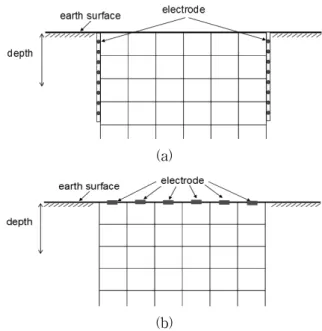
그림 2. 접지 저항 추정을 위한 전극 도면 (a) 대지 안쪽 에 놓여있는 전극, (b) 대지 표면에 놓인 전극 Fig. 2. Schematic diagram for subsurface resistance
estimation (a) array of electrodes placed inside the earth, (b) electrodes placed on earth surface.
where is the Jacobian of with respect to .
Jacobian is calculated based on sensitivity method[25]. Linearizing (23) about the resistivity vector at the
th iteration, we have
′ ≈ ′ ′′ (24)
Here, the term ′′ is the Hessian matrix, expressed as
′′ (25)
Substituting (23) and (25) in (24), we have the iterative solution for the resistivity update
(26)
Initial guess for the resistivity distribution inside the domain is calculated using least squares[22] as follows
(27)
where , and are constants. If we set to some value and compute the best resistivity value by minimizing the cost functional
∥
∥
(28)The solution to the above equation can be obtained as follows
(29)
Using the initial guess from (29) as the nominal or best resistivity value, the forward problem is solved and predicted voltages are compared with measured voltages. The resisitivity value is updated using (26) and the process is repeated until predicted voltages using FEM agree with measured voltages.
Ⅳ. Results and discussion
In this section, the results for the three- dimensional subsurface resistivity distribution using ERT are presented. The inverse algorithm is tested with numerical experiments.
1. Measurement setup
Soil resistivity can be measured through measurements by implanting the electrodes inside earth surface (borehole measurement). Another method is to have measurements from the electrodes placed on the top of the earth surface (surface measurement). The later method is economical as it does not involve the cost of making boreholes.
In this paper, using numerical simulations we have investigated the performance of ERT using measurem ents from all electrodes (two-side electrode) which can be visualized to that of borehole measurement and measurements using one-side electrode that can be compared to single borehole measurement or surface measurement (Fig. 2).
(a) (b)
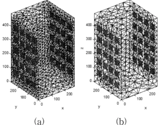
그림 3. FEM 정문제와 역문제 메쉬 (양측 전극면을 갖을 때). 전극은 표면의 빨간 부분임. (a) 조밀한 메쉬, (b) 성긴 메쉬
Fig. 3. Finite element mesh used in forward and inverse computations with two-side electrode measurement.
Electrodes are represented by red surface patches. (a) fine mesh, (b) coarse mesh.
(a) (b)
그림 4. FEM 정문제와 역문제 메쉬 (한쪽 전극면을 갖을 때). 전극은 표면의 빨간 부분임. (a) 조밀한 메쉬, (b) 성긴 메쉬
Fig. 4. Finite element mesh used in forward and inverse computations with one-side electrode measurement.
Electrodes are represented by red surface patches. (a) fine mesh, (b) coarse mesh.
Simulations are carried out using a test phantom that has geometry (280 mm × 280 mm × 490 mm) as shown in Fig. 3 and Fig. 4.
Stainless steel electrodes (40 mm × 40 mm) are placed on two opposite sides of the test phantom with 20 electrodes on each side. Neighboring electrodes are separated by a distance of 80 mm and 60 mm between the centers points vertically and horizontally, respectively, such that it comprises of five layers of electrodes with four electrodes in each layer. The lower edge of the bottom electrode is at a distance of 65 mm in each vertical array from the
bottom of the test phantom. Moreover, in each layer of horizontal array, the first and last electrodes are at a distance of 50 mm from the outer surface of the phantom. Two different meshes are used for forward and inverse solver so that inverse crime is avoided.
Fine mesh with 43581 nodes and 8473 tetrahedral elements are considered in generating the voltage data. In the inverse computation, coarse mesh with 7421 nodes and 1645 tetrahedral elements is used to estimate the internal resistivity distribution. In solving the inverse algorithm, best homogeneous resistivity is computed using (28).
2. Data acquisition
In ERT, image reconstruction depends on the selection of the current injection mechanism and the number of independent measurements that are available. In borehole measurement configuration (two-side electrode), single or multiple electrodes can be used as current driven pairs. In here, as a current injection protocol, opposite method is employed. A current of magnitude 10 mA is applied between the electrode on one surface and the corresponding opposite electrode on the other surface of the phantom. Resulting voltages are measured across the remaining 38 electrodes. Current carrying electrodes are not considered for measurement therefore for a single current injection 37 independent measurements are available. There are 20 possible current patterns for a 40 electrode configuration therefore a total number of 37 × 20 = 740 measurements are recorded for a single experiment.
In surface measurement configuration (one-side electrode), there are 20 electrodes with five layers of electrodes with 4 electrodes each. As a current injection protocol adjacent method is employed where neighboring electrodes are used as current driven pairs. Similarly, voltages are not measured at the surfaces of the current carrying electrodes. For a single current injection, 16 independent measurements are available therefore in single experiment with 20 electrode configuration, 16 × 20 = 320 measurements are available.
(a) (b) (c)
(d) (e)
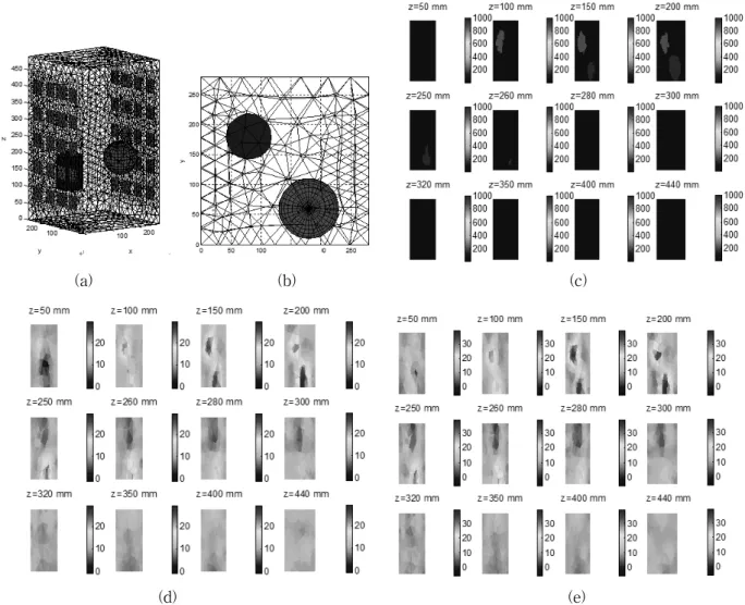
그림 5. 원통형 및 구형 타겟을 갖는 시뮬레이션 결과 (a) 시뮬레이션 타겟, (b) x-y 평면 상의 타겟 위치, (c) z축에 따른 실제의 저항률 분포 (d) z축에 따른 1번 반복 후 추정된 저항률 분포, (e) z축에 따른 5번 반복 후 추정된 저항률 분포.
Fig. 5. Simulation results with a cylindrical and spherical object inside the test phantom (a) targets used in simulation, (b) location of targets inside the test phantom, (c) true resistivity distribution, (d) estimated resistivity distribution after one iteration, (e) estimated resistivity distribution after five iterations. 2D plots sliced at different heights are shown here.
그림 6. 두 개의 타겟을 갖을 때 측정 전압과 계산 전압 의 norm 전압
Fig. 6. Norm voltage of measured and calculated voltages for synthetic data with two targets inside the phantom.
3. Results with Numerical data
For two-side electrode measurement, the synthetic data is generated by assuming a background resistivity of 10 mm and two resistive objects, cylinder (200 mm), sphere (1000 mm) located inside the phantom. Contact impedance value is set to 100 mm2.
There constructed results are shown in Fig. 5. Fig.
5(a-b) shows the target true size and location. The true resistivity values of the targets are given in Fig.
5(c). Estimated resistivity profile after single iteration with Gauss-Newton method is given in Fig. 5(d).
The target (cylinder, sphere) location and size are
(a) (b)
그림 7. 한쪽 전극 면을 갖을 때의 3가지 경우에 따른 시뮬레이션 결과 (a) x-y 평면 상의 타겟 위치, (b) z축에 따른 5번 반복 후 추정된 저항률 분포
Fig. 7. Simulation results for three-dimensional resistivity distribution with one-side electrodes. 2D plots obtained when sliced at different heights are given here. Target located at three positions is considered. (a) the true target location (b) the estimated resisivity profile obtained through iterating inverse algorithm five times.
그림 8. 한쪽 전극 면을 갖을 때의 3가지 경우에 대한 측정 전압과 계산 전압의 norm 전압
Fig. 8. Norm voltage of the measured and calculated voltages using synthetic data with one-side electrodes and spherical target inside the phantom.
detected with good accuracy. Also, it can be noticed that the estimated target resistivity values are less when compared to true resistivity value. This is the limitation of the inverse algorithm as the contrast ratio between the background and the target is very high. The resistivity values of the target and background are improved upon iterating the Gauss-Newton solution which can be noticed in Fig.
5(e). Norm voltage between the measured and calculated voltages is plotted in Fig. 6 and it can be noticed that norm voltage decreases with each iteration.
Synthetic data with one-side electrode measurement is tested with a spherical object of radius 38 mm placed at height 300 mm from the bottom of the test phantom. Sphere placed at three different locations in the x-y plane is investigated. In Fig. 7, the reconstructed results using Gauss-Newton after five iterations is given. Fig. 7(a) shows the true target location and Fig. 7(b) contains the resistivity profile corresponding to target position. Fig. 7 shows the estimated resistivity profile for case 1, where target is placed near to the boundary containing electrodes. Through the results it can be noticed that the target location and size is estimated well. As for case 2, spherical target is placed near the center of the x-y plane.
As seen from the Fig. 7, target location and size is detected with reasonable accuracy. In case 3, spherical target is placed very far from the electrode surface. The results show that the target is distinguishable even though it is far from the electrode. However, the target location is estimated little lower than the actual height. Sensitivity decreases as the distance between the target and electrode surface increase therefore, target resistivity values are estimated lesser when compared to the target which is located near the electrode surface. In Fig. 7, in obtaining the results regularization parameter of 7× e-4, 5×e-4, 5×e-4 is used, respectively.
Norm voltage for the three cases mentioned above is given in Fig. 8. In all the three cases, norm value is found to decrease with iteration.
Ⅴ. Conclusions
This paper presents an application of geophysics to determine the subsurface resistivity distribution using electrical resistance tomography. The resistivity distribution helps in designing an efficient earth grounding system. To survey the test location, conventional measurement techniques like four-point method are expensive, time consuming and cumbersome. Electrical resistance tomography which is relatively low cost offers fast measurements and presents three-dimensional resistivity plots. The reconstruction method is based on the finite element formulation of the forward model and as a nonlinear inverse solver iterated Gauss-Newton method is employed. Two kinds of measurement paradigm are studied which consider the use of two-side and one-side electrodes which can be associated to borehole and surface measurements. The results from synthetic and experimental studies reveal that electrical resistance tomography offers promising method to reconstruct the resisitivity distribution inside the subsurface and can assist in designing an efficient earth grounding grid.
REFERENCES
[1] P. Simonds, “Designing and testing low-resistance grounding systems,” IEEE Power Engineering Review, Vol. 20, no. 10, pp. 19-21, October 2000.
[2] N. H. Malik, A. A. Al-Arainy, M. I. Qureshi, M.
S. Anam, “Measurement of earth resistivity in different parts of Saudi Arabia for grounding installations,” in Proc. of seventh Saudi engineering conference, pp. 257-267, KSU, Riyadh.
[3] H. Yang, J. Yuan, W. Zong, “Determination of the-layer earth model from wenner four-probe test data,” IEEE Trans. Magnetics, Vol. 37, no.
5, pp. 3684-3687, September 2001.
[4] I. F. Gonos, V. T. Kontargyri, I. A. Stathopulos, A.X. Moronis, A.P. Sakarellos, N. I. Kolliopoulos,
“Determination of two layer earth structure parameters,” XVII International conference on Electromagnetic Disturbances EMD 2007, pp.
10.1-10.5, Poland.
[5] IEEE Std 81-1983., IEEE guide for measuring earth resistivity, ground impedance, and earth surface potentials of a ground system, 1983.
[6] A. M. Dijkstra, B.H. Brown, A. D. Leathard, N.
D. Harris, D. C. Barber, D. L. Endbrooke,
“Review clinical applications of electrical impedance tomography,” Journal of Medical Engineering and Technology, Vol. 17, no. 3, pp.
89-98, 1993.
[7] A. K. Khambampati, A. Rashid, U. Z. Ijaz, S.
Kim, M. Soleimani, K. Y. Kim, “Unscented Kalman filter approach to track moving interfacial boundary in sedimentation process using three-dimensional electrical impedance tomography,” Philosophical Transactions of Royal Society A, Vol. 367, no. 1900, pp. 3095-3120, July 2009.
[8] D. H. Griffiths and R.D. Barker, “Two-dimensional resistivity imaging and modeling in areas of complex geology,” Journal of applied geophysics, Vol. 29, no. 3-4, pp. 211-226, April 1993.
[9] K. A. Dines and R. J. Lytle, “Analysis of electrical conductivity imaging,” Geophysics, Vol.
46, no. 7, pp. 1025-1036, July 1981.
[10] W. Daily, A. Ramirez, R. Johnson, “Electrical impedance tomography of a perchloroethelyne release,” Journal of Environmental and Engineering Geophysics, Vol. 2, no. 3, pp.
189-201, 1998.
[11] R. D. Barker, J. Moore, “The application of time-lapse electrical tomography in groundwater
studies,” Leading Edge, Vol. 17, no. 10, pp.
1454-1458, October 1998.
[12] W. Daily and A. Ramirez, “Electrical resistivity tomography of vadose water movement,” Water Resource Research, Vol. 28, no. 5, pp. 1429-1442, 1992.
[13] B. Spies and R. Ellis, “Cross-borehole resistivity tomography of a pilot scale, insitu verification test,” Geophysics, Vol. 60, no. 3, pp. 886-898, May-June 1995.
[14] A. Casas, M. Himi, Y. Diaz, V. Pinto, X. Font, J.C. Tapias, “Assessing aquifer vulnerability to pollutants by electrical resistivity tomography (ERT) at a nitrate vulnerable zone in NE Spain,” Environmental Geology, Vol. 54, no. 3, pp. 515-520, April 2008.
[15] L. N. Meads, L. R. Bently, C.A. Mendoza,
“Application of electrical resistivity imaging to the development of a geological model for a proposed Edmonton landfill site,” Canadian Geotechnical Journal, Vol. 40, no. 3, pp. 499-523, June 2003.
[16] A. L. Ramirez, D. A. Chesnut, W.D. Daily,
“Using electrical resistance tomography to map subsurface temperatures,” US patent No.
5346307, 1994.
[17] B. S. Kim, S. Kim, K. Y. Kim, “Development of Novel on-line Landweber Algorithm for Image Reconstruction in Electrical Impedance Tomography” Journal of the Institute of Electronics Engineers of Korea, Vol. 49, no. 9, pp. 293-299, September 2012.
[18] K. Y. Kim, B. S. Kim, S. I. Kang, M. C. Kim, J. H. Lee, Y. J. Lee, “Dynamical Electrical Impedance Tomography Based on the Regularized Extended Kalman Filter” Journal of the Institute of Electronics Engineers of Korea, Vol. 38, no. 5, pp. 23-32, September 2001.
[19] K. Y. Kim, B. S. Kim, M. C. Kim, Y. J. Lee, M.
Vauhkonen, “Image reconstruction in time varying electrical impedance tomography based on the extended Kalman filter,” Measurement Science Technology, Vol. 12, no. 8, pp.
1032-1039, April 2001.
[20] A. K. Khambampati, A. Rashid, J. S. Lee, B. S.
Kim, L. Dong, S. Kim, K. Y. Kim, “Estimation of void boundaries in flow field using expectation maximization algorithm,” Chemical Engineering Science, Vol. 66, no. 3, pp. 355-374, February 2007.
[21] M. Gasulla, R. Pallas-Arney, “Noniterative algorithms for electrical resistivity imaging
저 자 소 개 Anil Kumar Khambampati(Member)
2003 BS degree in Mechanical Engineering, Jawaharlal Nehru Technological University, India 2006 MS degree in Marine Instrumentation Engineering, Jeju National University
2010 PhD degree in Electronic Engineering, Jeju National University
<Research interests : Inverse problem, Electrical tomography, Optimal Control>
Kyung Youn Kim(Member) 1983 BS degree in Electronic Engineering, Kyungpook National University
1986 MS degree in Electronic
Engineering, Kyungpook
National University
1990 PhD degree in Electronic Engineering, Kyungpook National University
<Research interests : Inverse problem, Electrical tomography, Instrumentation & Control>
applied to subsurface local anamolies,” IEEE Sensors Journal, Vol. 5, no. 6, pp. 1421-1432, December 2005.
[22] P. J. Vauhkonen, M. Vauhkonen, T. Savolainen, J.P. Kaipio, “Three-dimensional electrical impedance tomography based on the complete electrode model,” IEEE Transactions on Biomedical Engineering, Vol. 46, no. 9, pp.
1150-1160, September 1999.
[23] O. P. Tossavainen, M. Vauhkonen, V.
Kolehmainen, “A three-dimensional shape estimation approach for tracking of phase interfaces in sedimentation processes using electrical impedance tomography,” Measurement Science and Technology, Vol. 18, no. 5, pp.
1413-1424, March 2007.
[24] O. P. Tossavainen, V. Kolehmainen, M.
Vauhkonen, “Free surface and admittivity estimation in electrical impedance tomography,”
International Journal of Numerical Methods and Engineering, Vol. 66, no.13, pp. 1991-2013, June 2006.
[25] M. Cheney, D. Isaacson, J.C. Newell, S. Simke, J. Goble, “NOSER: An algorithm for solving the inverse conductivity problem,” International Journal of Imaging Systems and Technology, Vol. 2, no. 2, pp. 66-75, 1990.